
Models of Earth's Interior
(i.e., characterizing the interior from either seismic data, or computer calculations of convective motions, etc.)
|
Some Images Relating to Models of Earth's interior (return to image directory page)
|
||||
 |
 |
 |
 |
 |
| AI (3.2 Mb) JPG (450 Kb) | AI (3.9 Mb) JPG (388 Kb) | AI (1.0 Mb) JPG (471 Kb) | AI (1.6 Mb) JPG (397 Kb) | AI (1.2 Mb) JPG (322 Kb) |
|
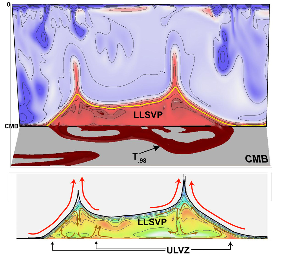
Here we start off with a geodynamics prediction for a chemically distinct pile of material at the base of Earth's mantle, from Allen McNamara. This figure was made to emphasize that these "Large Low Shear Velocity Provinces" (LLSVPs) may have really interesting internal convection [PDF]
|
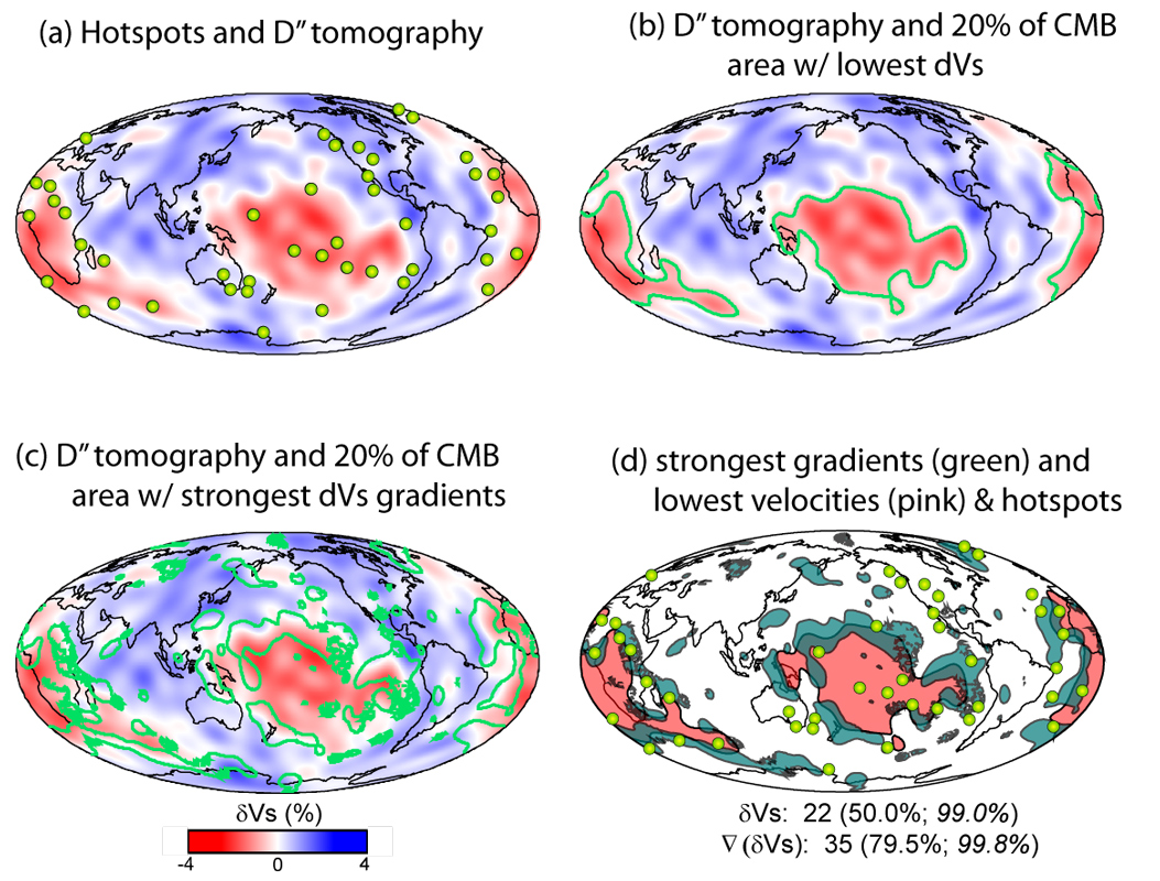
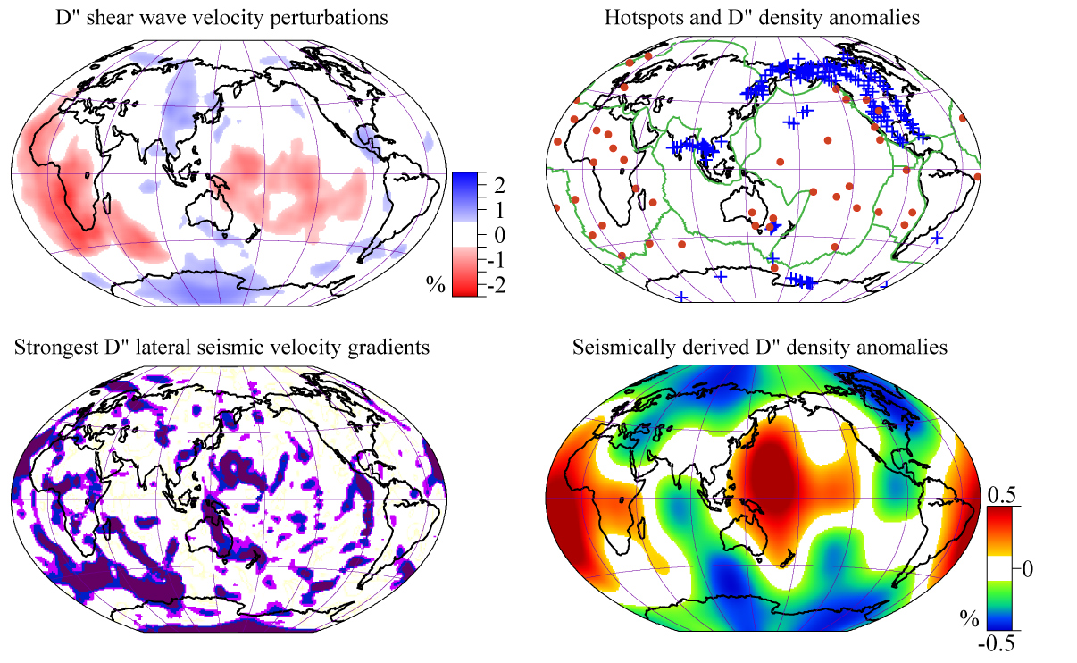
Mike Thorne's 2004 paper (PDF) demonstrated that hot spots are nearly twice as likely to overly the edges of the large low shear velocity provinces in the deep mantle (as measured by lateral Vs gradients) than the low velocities themselves. We argued this is evidence for a chemical nature to the regions.
|
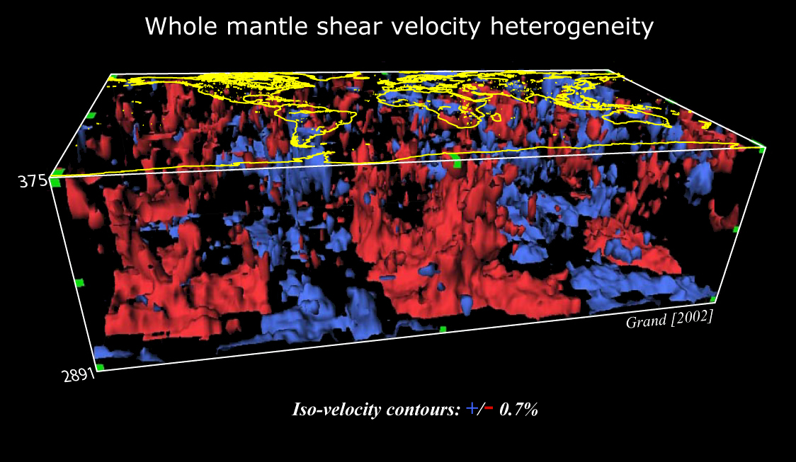
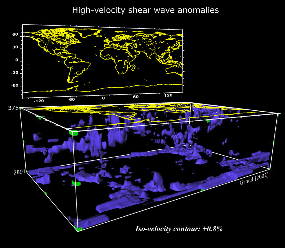
These blobs are due to iso-surfacing shear velocity perturbations throughout Earth's mantle. Here it is done with Steve Grand's model from 2002.
|
Iso-surfacing programs are really fun. Here, I just show the highest velocities, to hunt for subducted slabs. By the way, an amazing freeware program that does this is called "Data Explorer", or DX. Go HERE to see and explore. Allen is our resident expert at it, and keeps telling me to learn it.
|
|
|
Some Images Relating to Models of Earth's interior (return to image directory page)
|
||||
 |
 |
 |
 |
 |
| AI (522 Kb) JPG (543 Kb) | AI (693 Kb) JPG (627 Kb) | AI (2.1 Mb) JPG (754 Kb) | AI (875 Kb) JPG (629 Kb) | AI (398 Kb) JPG (452 Kb) |
|
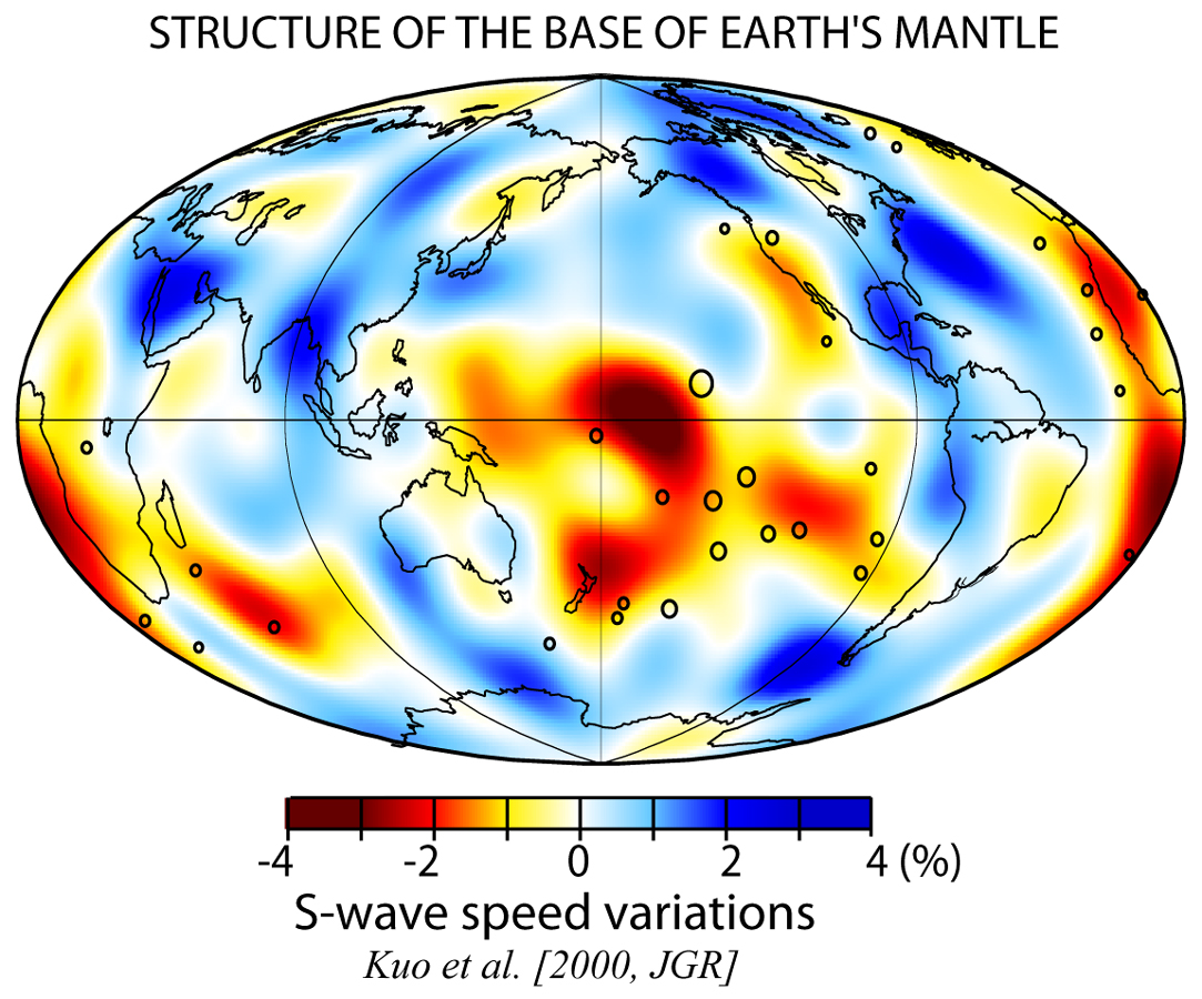
The shear velocity in the deep mantle is determined globally from tomography. This paper was led by Ban Kuo. It employed a 2-step approach: (1) low order spherical harmonic inversion, and (2) smaller scale block inversion. [PDF]. Be sure to check out Allen's Spherical Harmonics page!
|
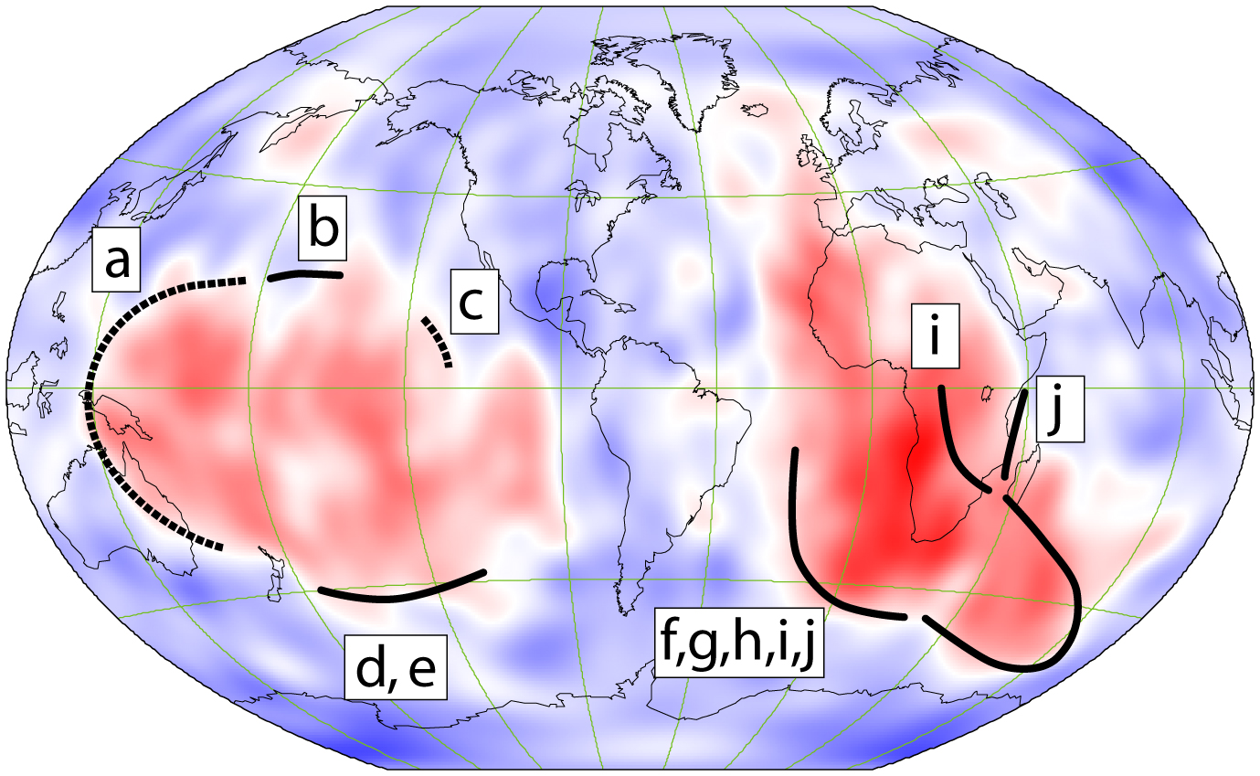
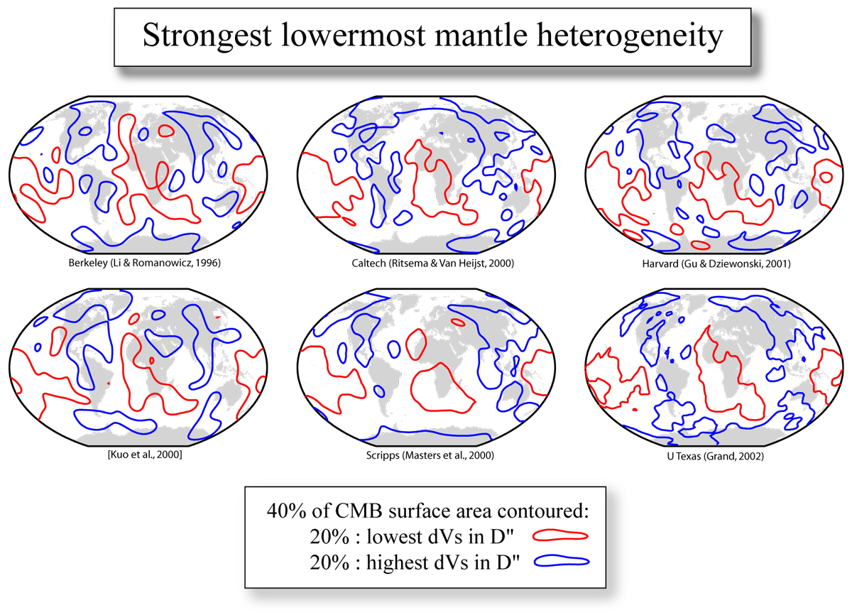
Have you heard the news lately? The large low shear velocity provinces in the deep mantle have sharp edges! (the black lines above). That supports the notion that the low shear velocities owe their existence in part to being chemically distinct from the rest of the mantle. [PDF]
|
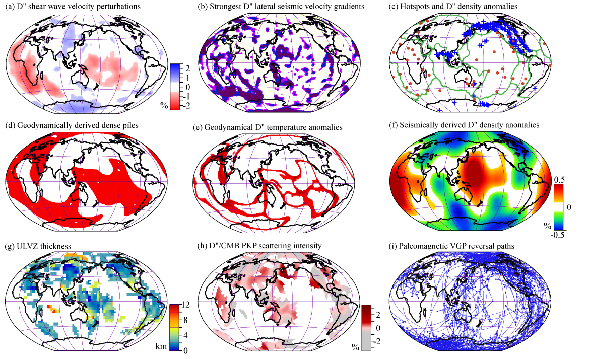
This figure is a busy as it gets... But there are some remarkable correlations between seismic, geodynamic, geochemical, and geomagnetic studies. Please refer to the paper that discusses these phenomena [PDF]. Multidisciplinary approaches are the only way to sort these things out.
|
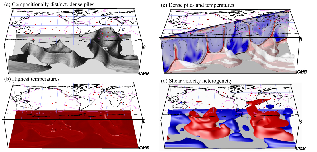
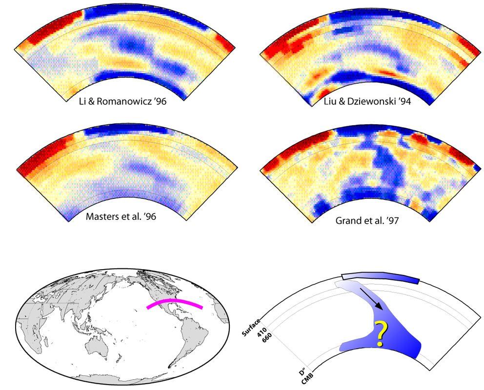
Here we show just 4 of the 9 panels of the image to the left. Can you see the correlations?
|
This is an old image, but I still see it getting used, so I'll leave it posted. Are the cross-sections showing us that slabs descend all the way down to the core-mantle boundary?
|
|
Some Images Relating to Models of Earth's interior (return to image directory page)
|
||||
 |
 |
 |
 |
 |
| AI (995 Kb) JPG (293 Kb) | AI (1.1 Mb) JPG (296 Kb) | AI (2.7 Mb) JPG (485 Kb) | AI (1.3 Mb) JPG (594 Kb) | AI (5.4 Mb) JPG (774 Kb) |
|
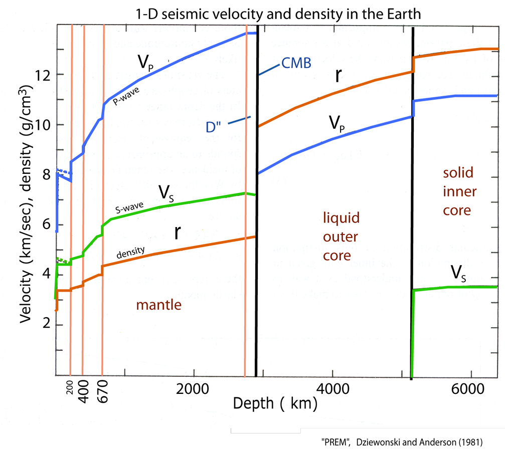
The Preliminary Reference Earth Model (PREM), by Dziewonski and Anderson (1981, Phys. Earth Planet. Int). Look at the next step REM page by Gabi Laske. This is the most used 1D model of seismic values. Here is PREM in ASCII and in Microsoft's EXCEL
|
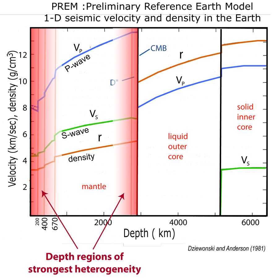
PREM again. This emphasizes where in Earth we have the greatest heterogeneities: at the top and bottom of the mantle. Here's a PowerPoint file that shows PREM (upper left), then the above image.
|
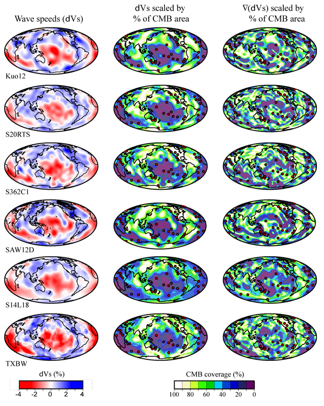
Here's another way Mike Thorne developed to look at tomography models (D" is shown here): scale the heterogeneity and lateral gradients of it by area. This then permits direct comparison of models (of different amplitudes) from different researchers. [PDF]
|
I compare 6 shear velocity models of D" to each other, using the area scaling approach (as in the figure to the left). Do they agree?
|
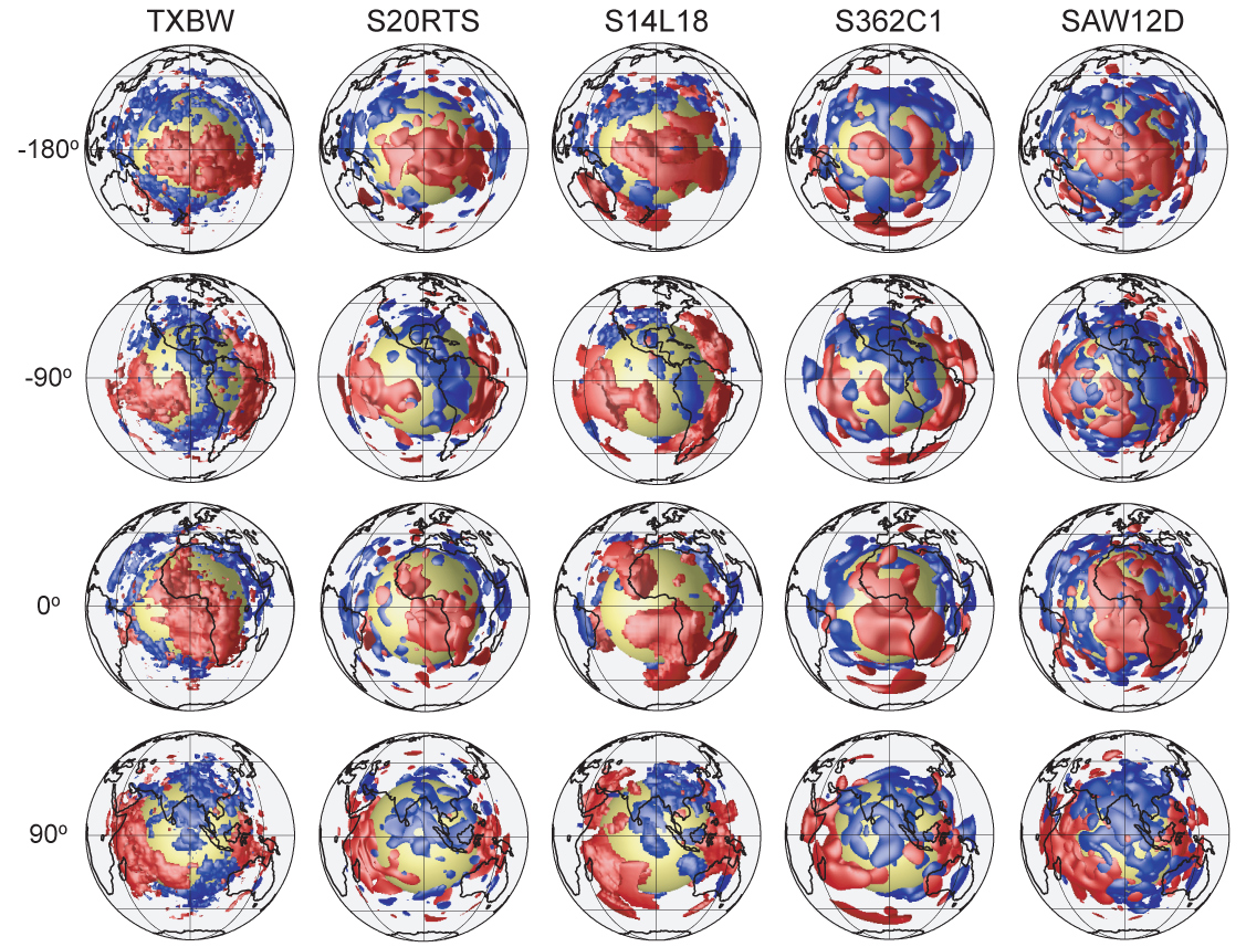
Using iso-surfacing, shear velocity perturbations are shown from 5 different researchers, with different rotations of the globe. I think at this type of scale, the models agree pretty well.
|
|
Some Images Relating to Models of Earth's interior (return to image directory page)
|
||||
 |
 |
 |
 |
 |
| AI (4.3 Mb) JPG (622 Kb) | AI (992 KMb) JPG (344 Kb) | AI (840 Kb) JPG (422 Kb) | AI (4.3 Mb) JPG (649 Kb) | AI (4.4 Mb) JPG (624 Kb) |
|
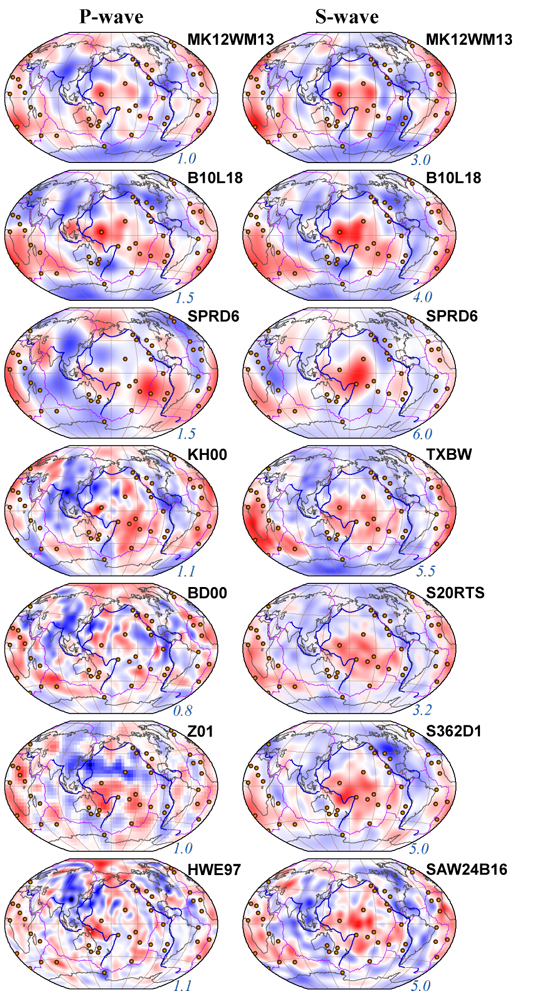
After all the previous images in 3D, this probably looks boring and old fashioned. NOT! Anyway, 7 P-wave models and 7 S wave models are shown, from PDF. I have to admit, Thorsten Becker gave me many of the models, from his nice paper comparing tomography models.
|
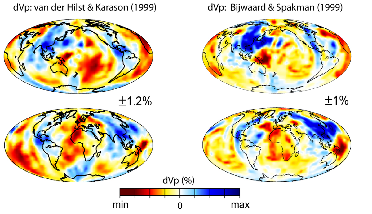
Just another view of the same thing, P models are shown here, from an older review paper.
|
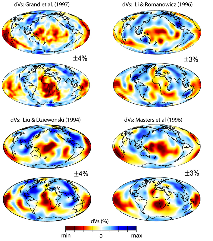
The same, but S-wave models from the same older review paper.
|
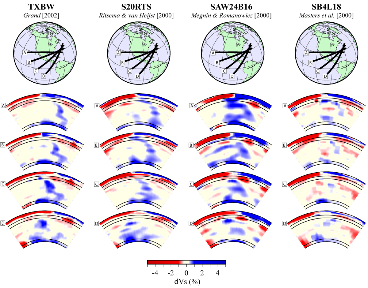
Where's Waldo? Or, rather, the slab? I think these cross-sections so pretty compelling evidence for high seismic wave speeds extending from a subduction zone to the CMB. Perhaps fuzzy here and there, especially to the south. Is the slab gone? or is our ability to see it gone?
|
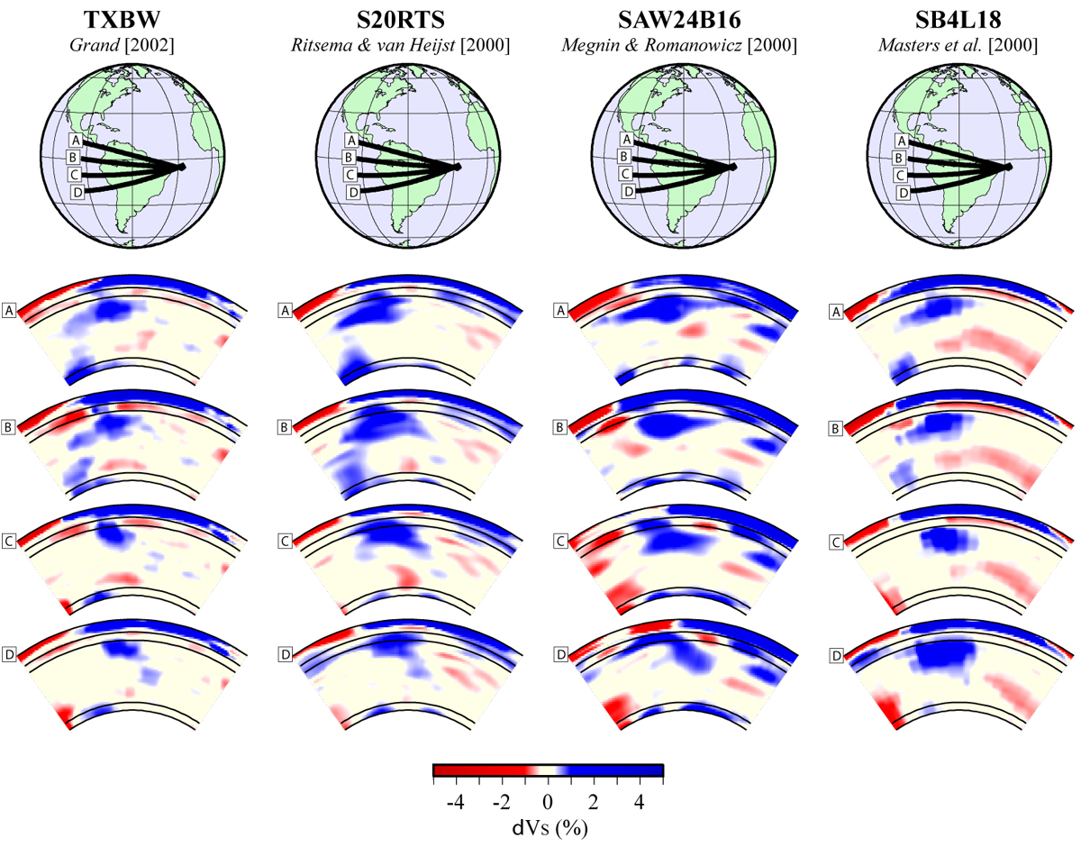
Here I show the same thing, but for northern South America. Take a look. The story may not be so clear here.
|
|
Some Images Relating to Models of Earth's interior (return to image directory page)
|
||||
 |
 |
 |
||
| AI (169 Kb) JPG (169 Kb) | AI (215 Kb) JPG (247 Kb) | AI (4.3 Mb) JPG (765 Kb) | ||
|
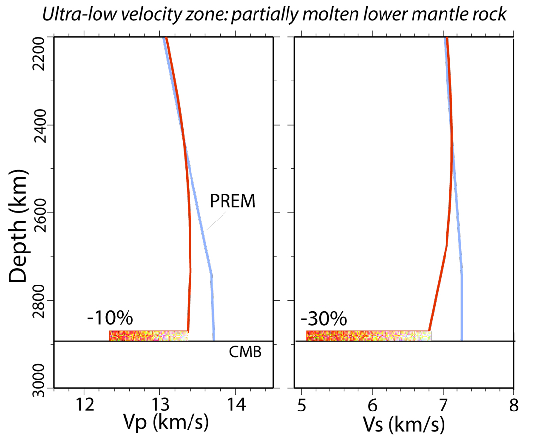
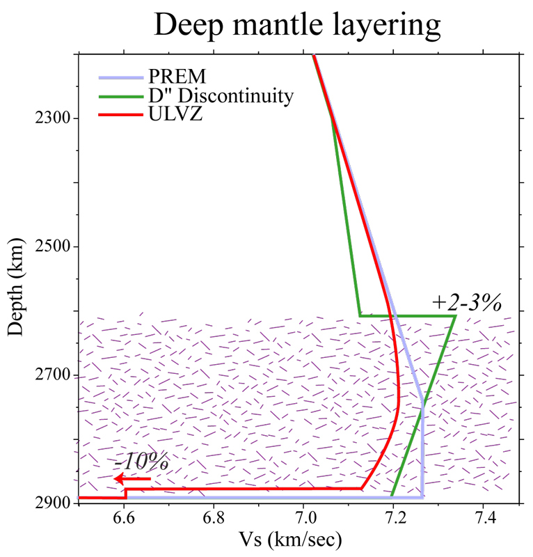
Here is a garden variety image of lowermost mantle seismic phenomena, including a D" discontinuity, and an Ultra-Low Velocity Zone. Here's a PowerPoint vingette showing similar things: PowerPoint File
|
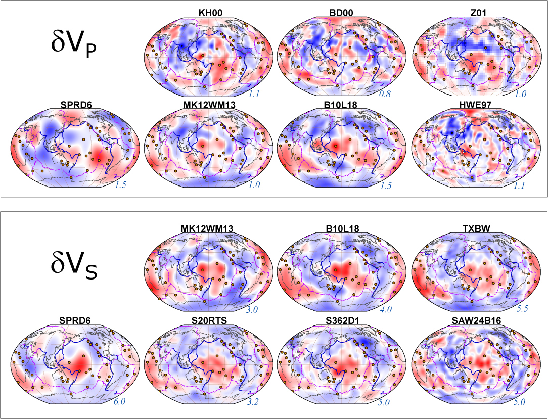
P and S models of the lowermost mantle again. This may actually be the same as an image above, but shifted around...
|
|
|
|