
"Seismology 101" images
|
Introduction to seismology images (return to image directory page)
|
||||
 |
 |
 |
 |
 |
| JPG (210 Kb) | JPG (183 Kb) | JPG (257 Kb) | JPG (166 Kb) | JPG (275 Kb) |
|
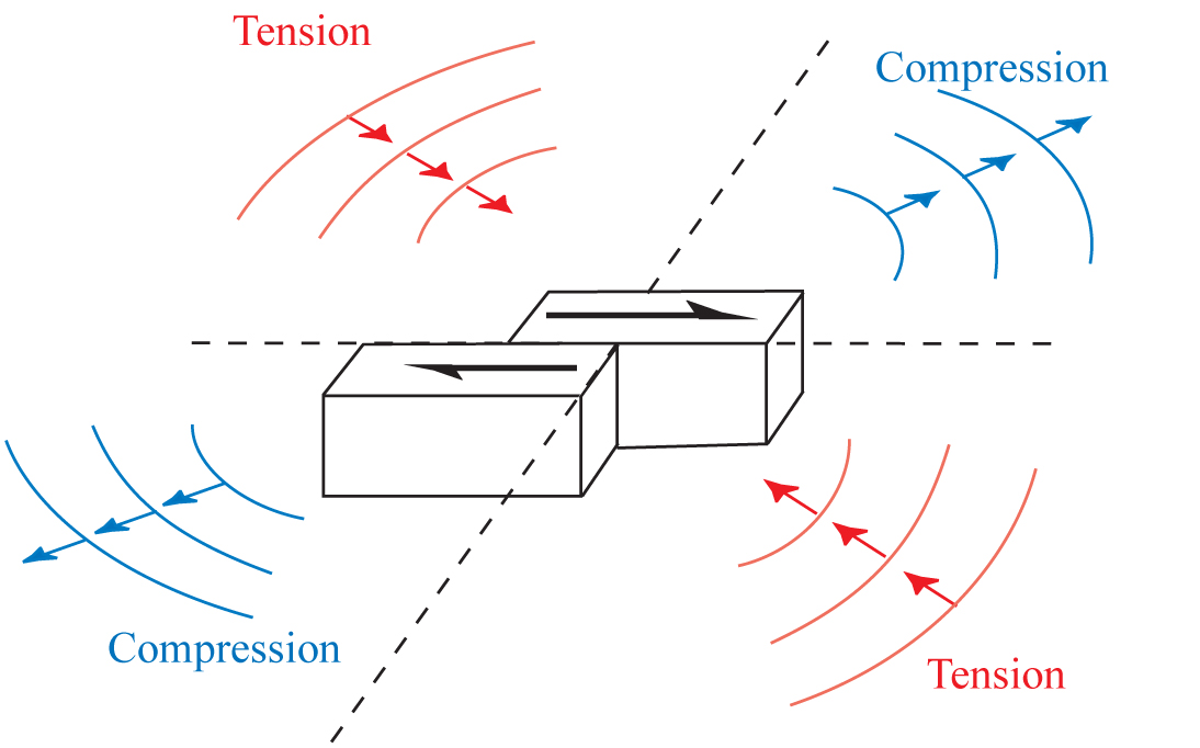
Strike-slip fault and compression and tension patterns seen in the far-field. [Apologies: I somehow lost my original artwork files for these focal mechanism images!]
|
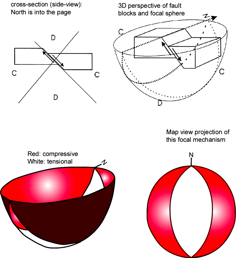
A reverse fault and compression (C) and tension (or, dilatation "D") patterns, and the resulting focal mechanism (red = compression). NOTE: this image and others slightly misrepresent the lower hemisphere projection in the 3D perspective views,; they solely intend to help the viewer see the lower hemisphere projection of the "beachball" which is usually first incorrectly interpreted by students to pop out of the page.
|
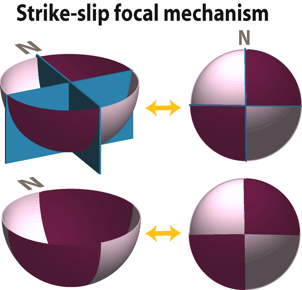
More views of a pure strike slip mechanism. NOTE: on this page I am showing focal mechanism information for the P-wave field. See also:
FOCAL MECHANISM and FOCAL MECHANISM PRIMER |
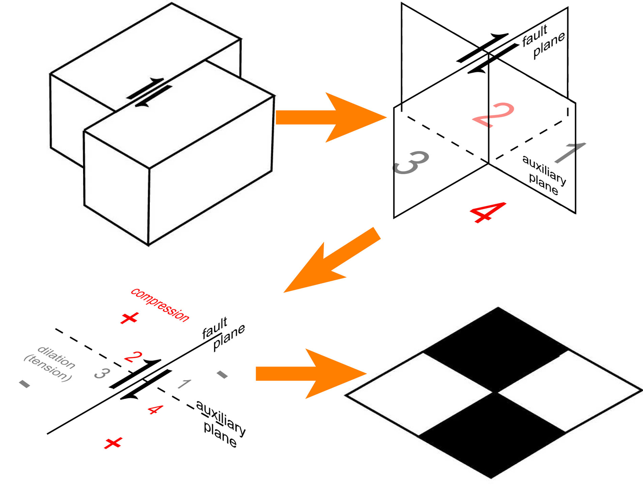
Strike-slip again, this time with blocks and planes. See also:
FAULT BLOCK FAULT TYPES |
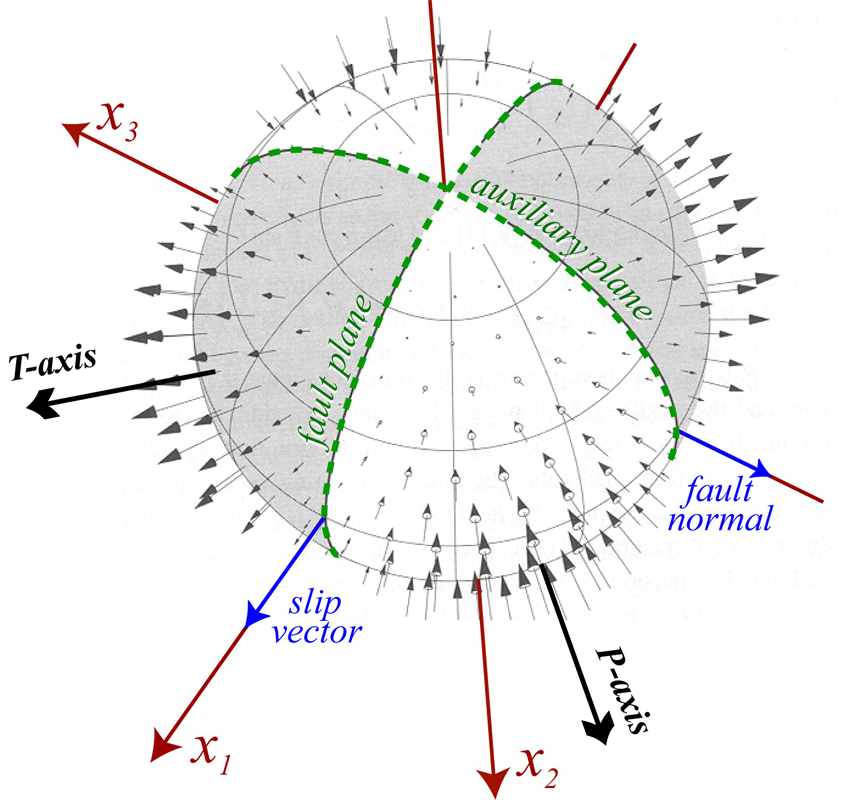
This modifies what I think is the coolest image out of Peter Shearer's book, Introduction to Seismology, a must buy if you don't have it. Here, we view the whole focal sphere. I've drawn in the possible fault and auxiliary plane, and P and T axes, coordinate system, etc. Did he do this in GMT?
|
|
Introduction to seismology images (return to image directory page)
|
||||
 |
 |
 |
 |
 |
| JPG (279 Kb) | AI (147 Kb) JPG (72 Kb) | AI (149 Kb) JPG (138 Kb) | AI (125 Kb) JPG (69 Kb) | AI (149 Kb) JPG (64 Kb) |
|
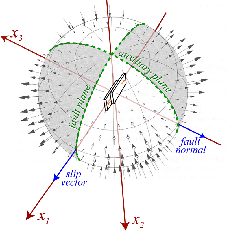
Again, doctoring up Peter's image, but this time, in the style of Hiroo Kanimori's old lecture notes, I put a mini-fault blocks slipping in the center of the sphere that could give rise to this amplitude field.
|
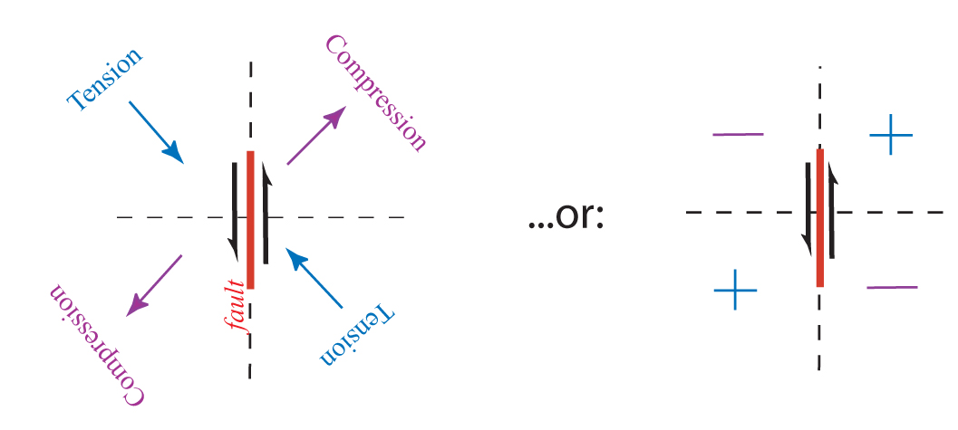
More on slip at the fault and compression or dilatation that we see in the far field.
|
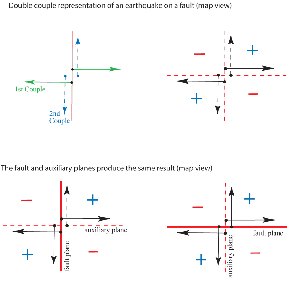
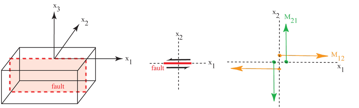
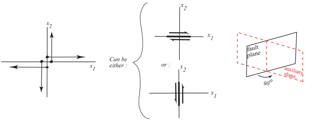
This is a "double couple" representation of slip on a fault. ...that is, a double force couple. Here we should that the fault plane has two possible positions which give the same far-field motions.
|
More on the double couple representation, from fault blocks to the two pairs of force couples.
|
I know, these get redundant. Oh well. This defines the fault and auxiliary planes.
|
|
Introduction to seismology images (return to image directory page)
|
||||
 |
 |
 |
 |
|
| AI (138 Kb) JPG (162 Kb) | AI (162 Kb) JPG (132 Kb) | AI (176 Kb) JPG (96 Kb) | AI (211 Kb) JPG (215 Kb) | AI (184 Kb) JPG (186 Kb) |
|
Just another graphical representation of what happens in the far-field.
|
Motions in the far-field vary as a function of distance to the nodal planes (fault and auxiliary planes) in a systematic fashion.
|
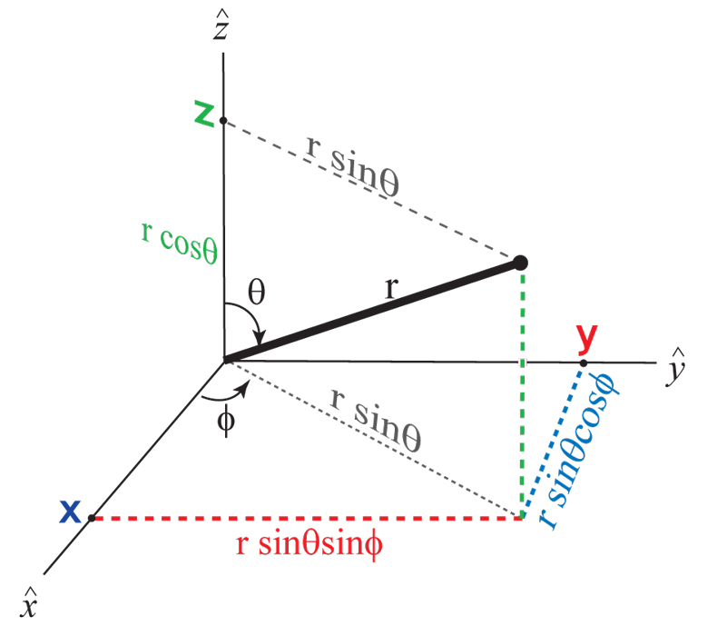
Seismologists often go between coordinate systems (Cartesian to Spherical, etc.). This image is pretty basic, but perhaps useful for teaching. I know... it is also out of place.
|
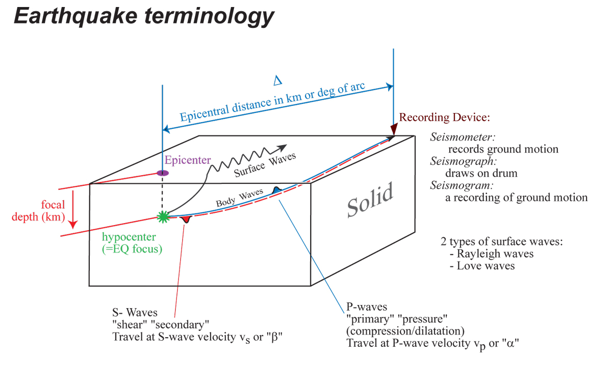
Here are some really general earthquake terms defined.
|
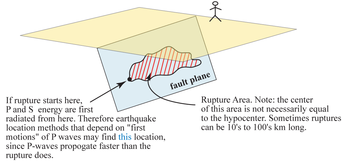
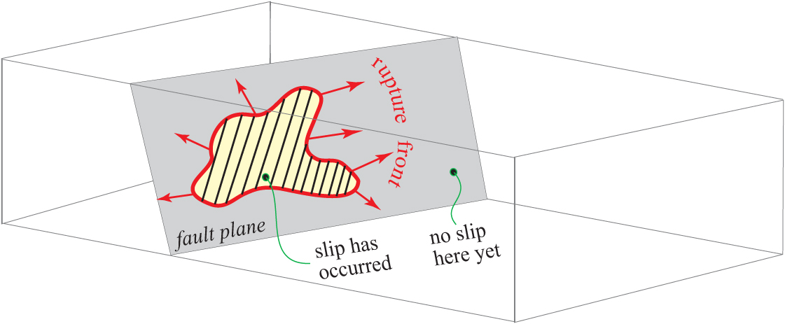
Here, the concept of rupture area, plane, and initiation are introduced. See also:
EARTHQUAKES |
|
Introduction to seismology images (return to image directory page)
|
||||
 |
 |
 |
 |
 |
| AI (150 Kb) JPG (122 Kb) | AI (164 Kb) JPG (126 Kb) | AI (164 Kb) JPG (193 Kb) | AI (200 Kb) JPG (320 Kb) | AI (116 Kb) JPG (40 Kb) |
|
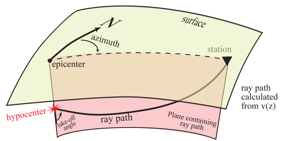
Some path geometry parameters are introduced here.
|
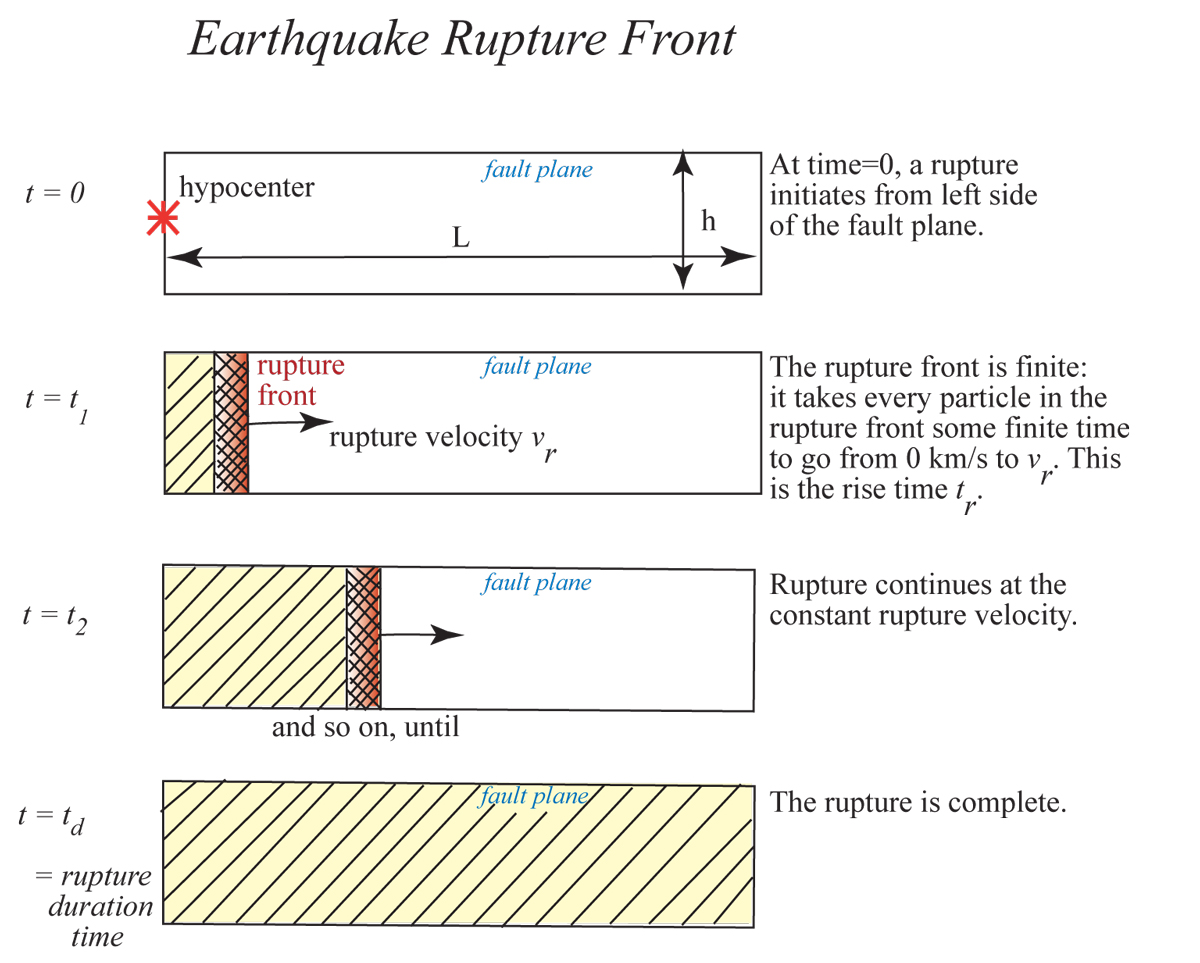
Here we introduce the concept of time during a rupture: it is a dynamic process that starts somewhere, then propagates out from that point. (Keep in mind this is a cartoon of a model of the earthquake process).
|
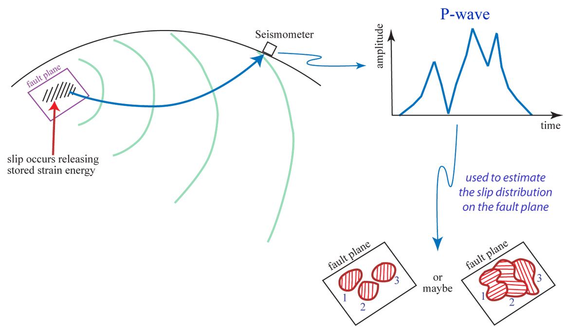
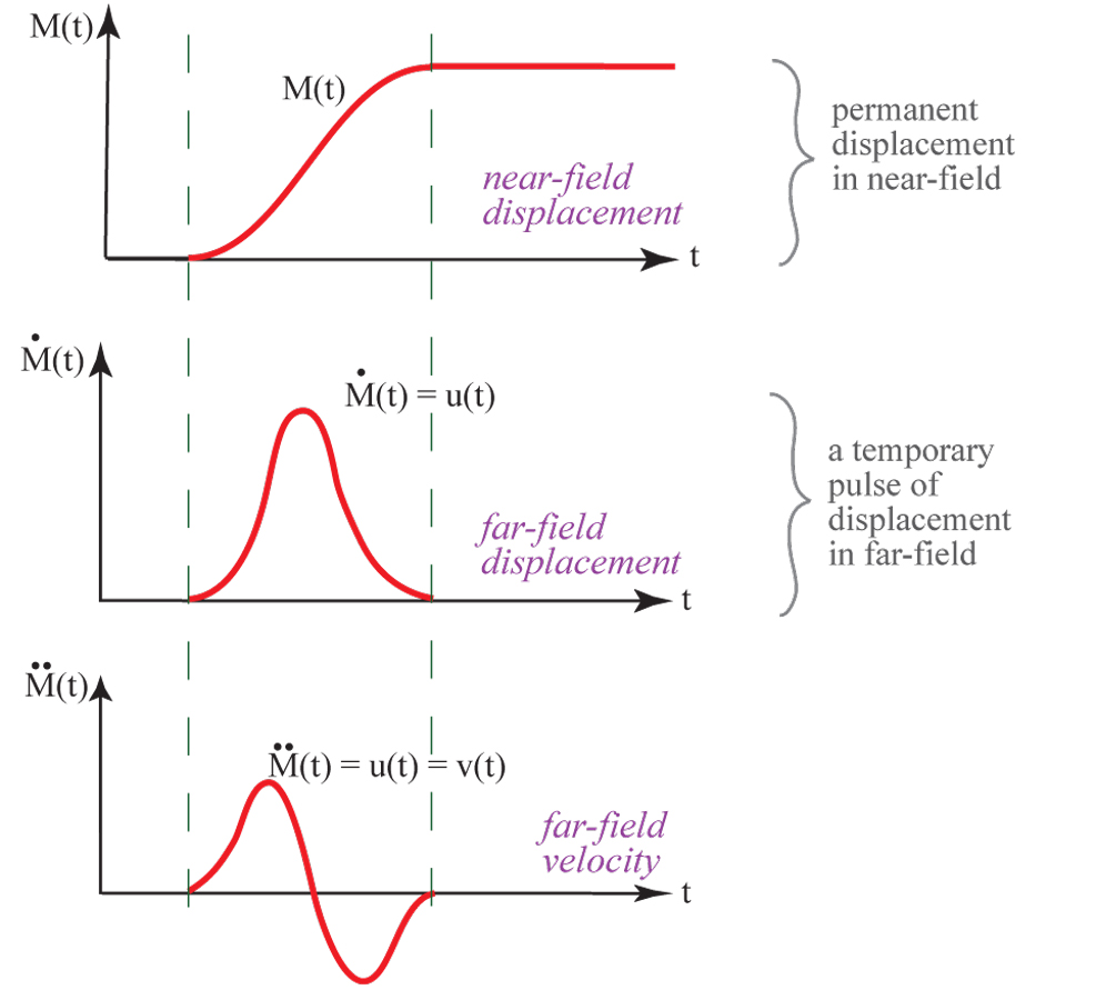
Far away from earthquakes, we have information about the earthquake process in the ground motion we observe. This shows a couple possibilities for the cartoon P-wave motion in the upper right.
|
Here is a depiction of how an area of fault might break.
|
Seismologists frequently use the mathematical operation of convolving two functions together. Ground motion at some distant place from an earthquake can be represented as a convolution of the earthquake source with the "path" operator with the seismic instrument response.
|
|
Introduction to seismology images (return to image directory page)
|
||||
 |
 |
 |
 |
 |
| AI (171 Kb) JPG (113 Kb) | AI (132 Kb) JPG (109 Kb) | AI (264 Kb) JPG (218 Kb) | AI (151 Kb) JPG (235 Kb) | AI (174 Kb) JPG (210 Kb) |
|
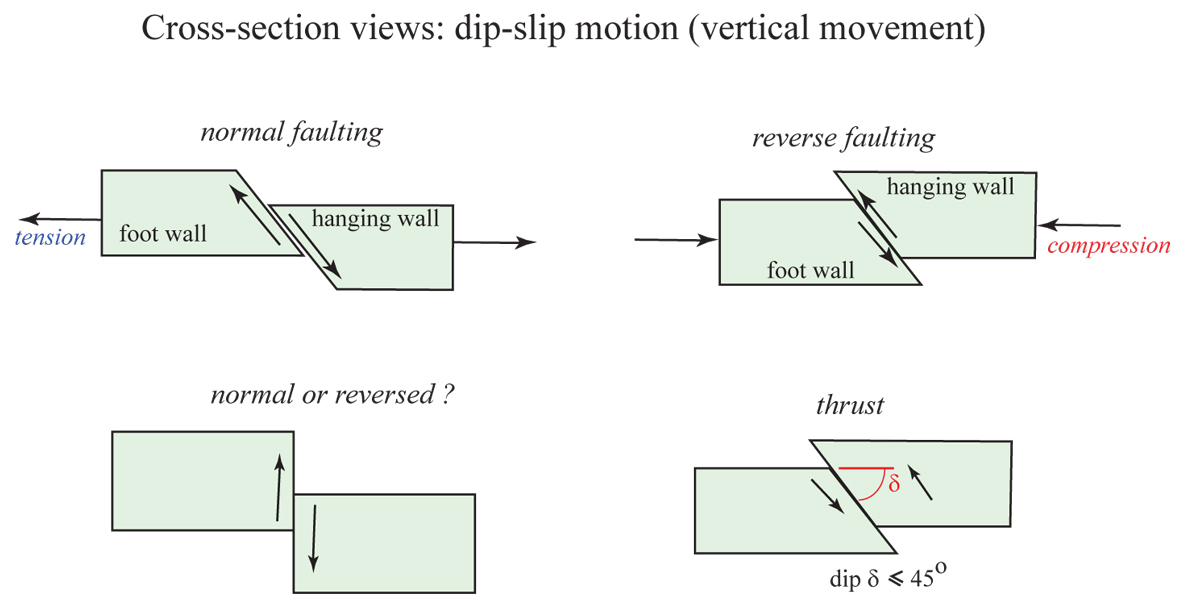
Here are some basic definitions of fault types. See also:
FAULT TYPES |
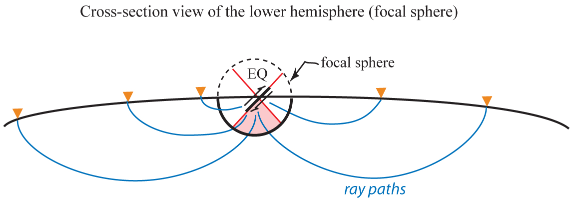
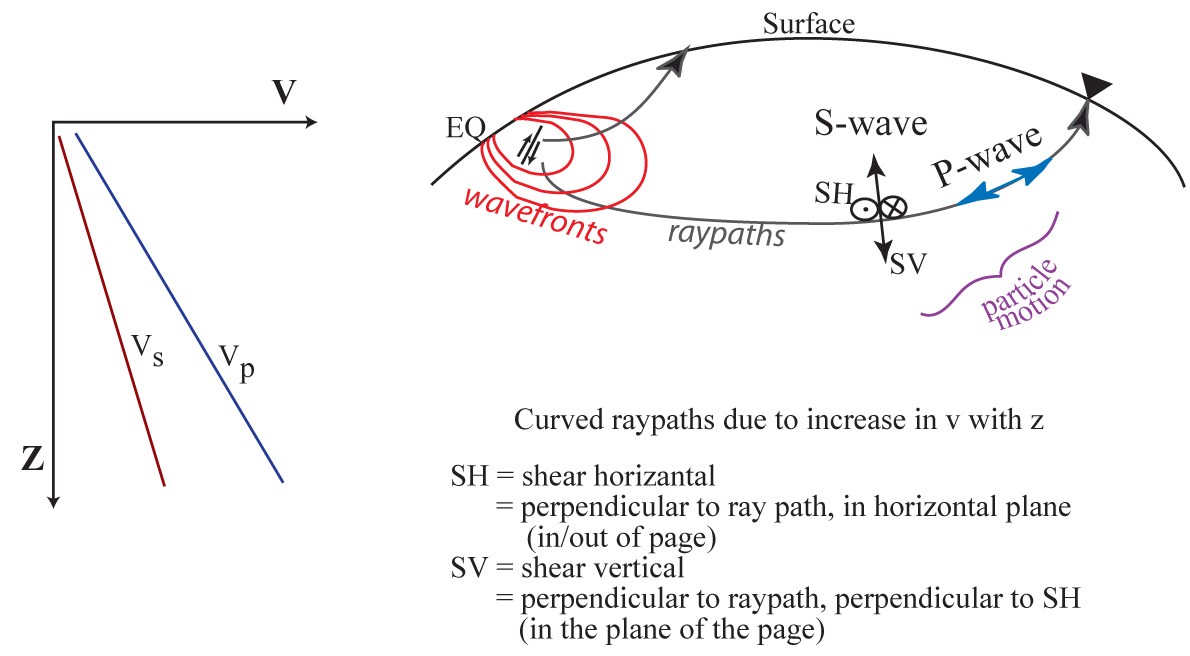
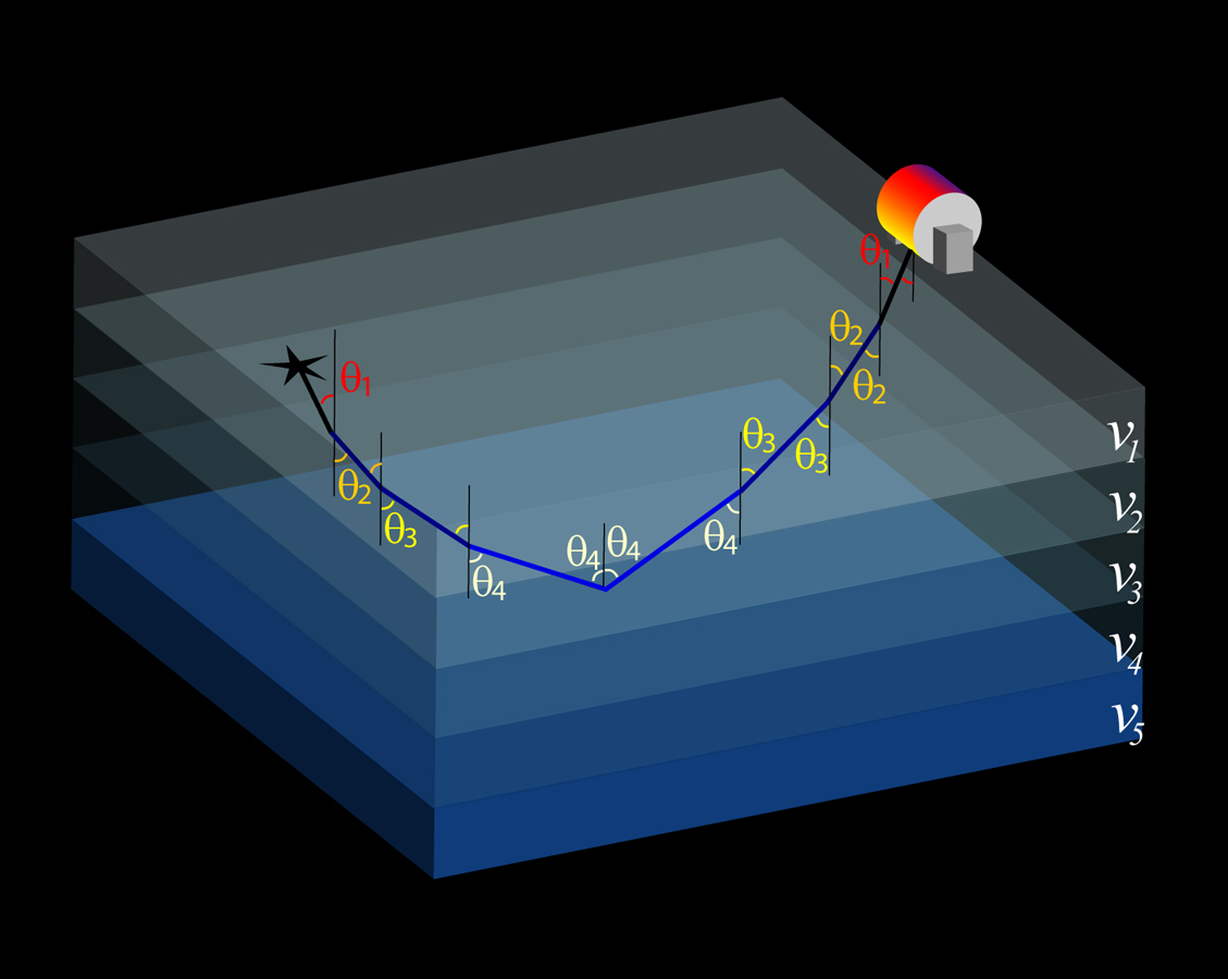
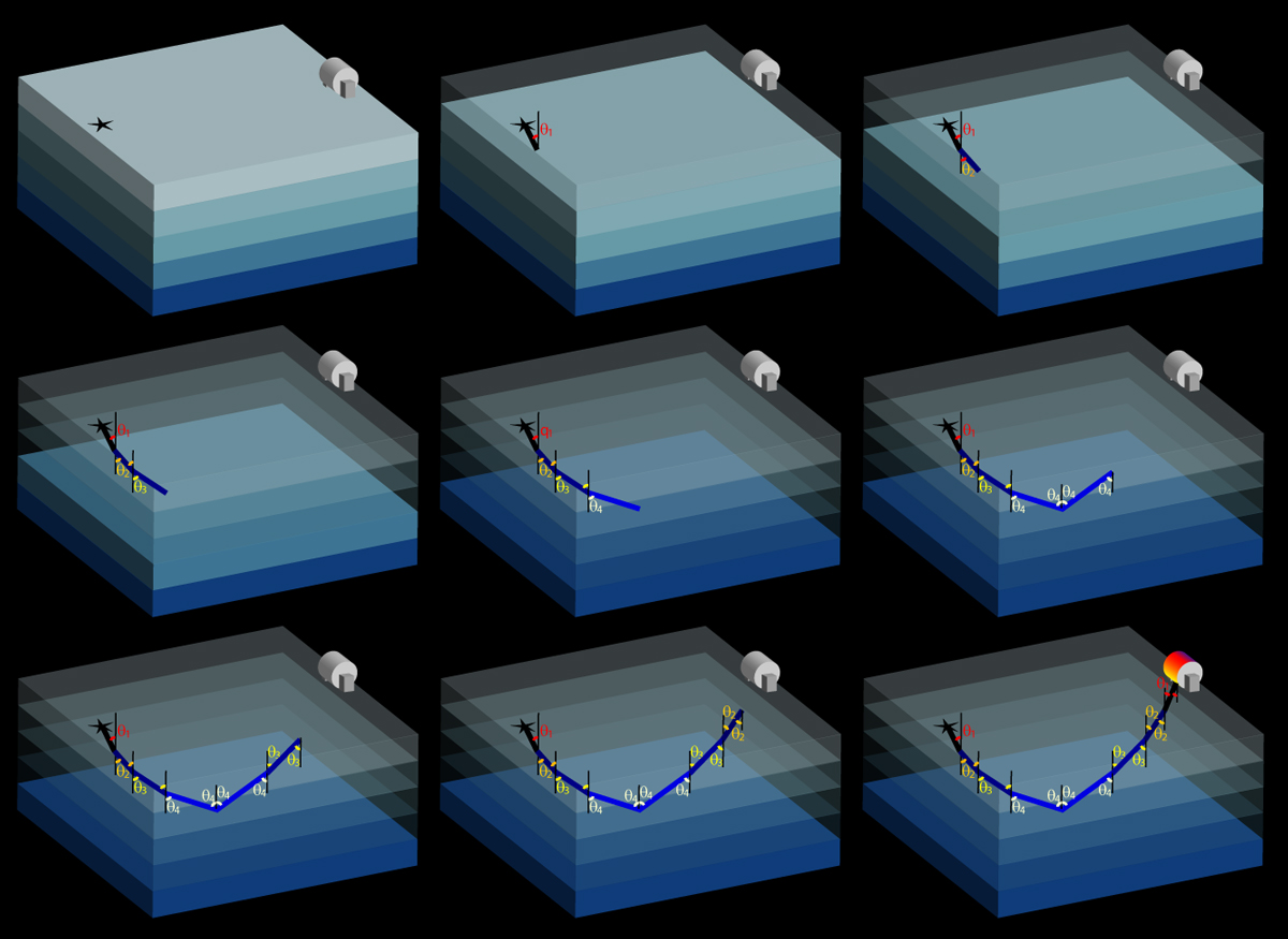
This is a side-view of a lower hemisphere focal mechanism, and shows idealized ray paths leaving the source area to distant recorders. The ray paths are curved because seismic velocity generally increases with depth in the Earth.
|
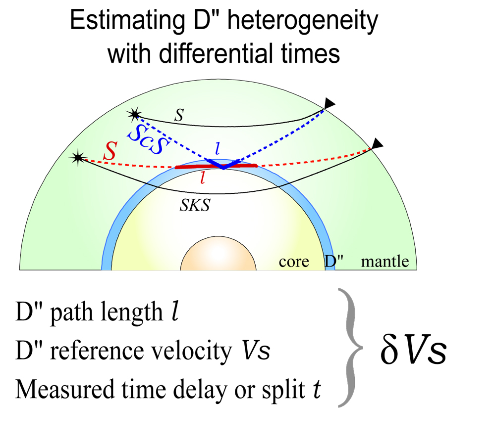
This cartoon shows one way that seismologists infer seismic velocity heterogeneities in the Earth from observed travel time variations.
|
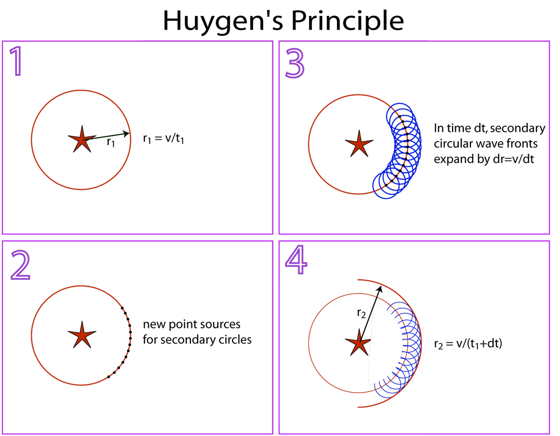
Huygens principle is illustrated here. See also:
HUYGENS-FRESNEL PRINCIPLE |
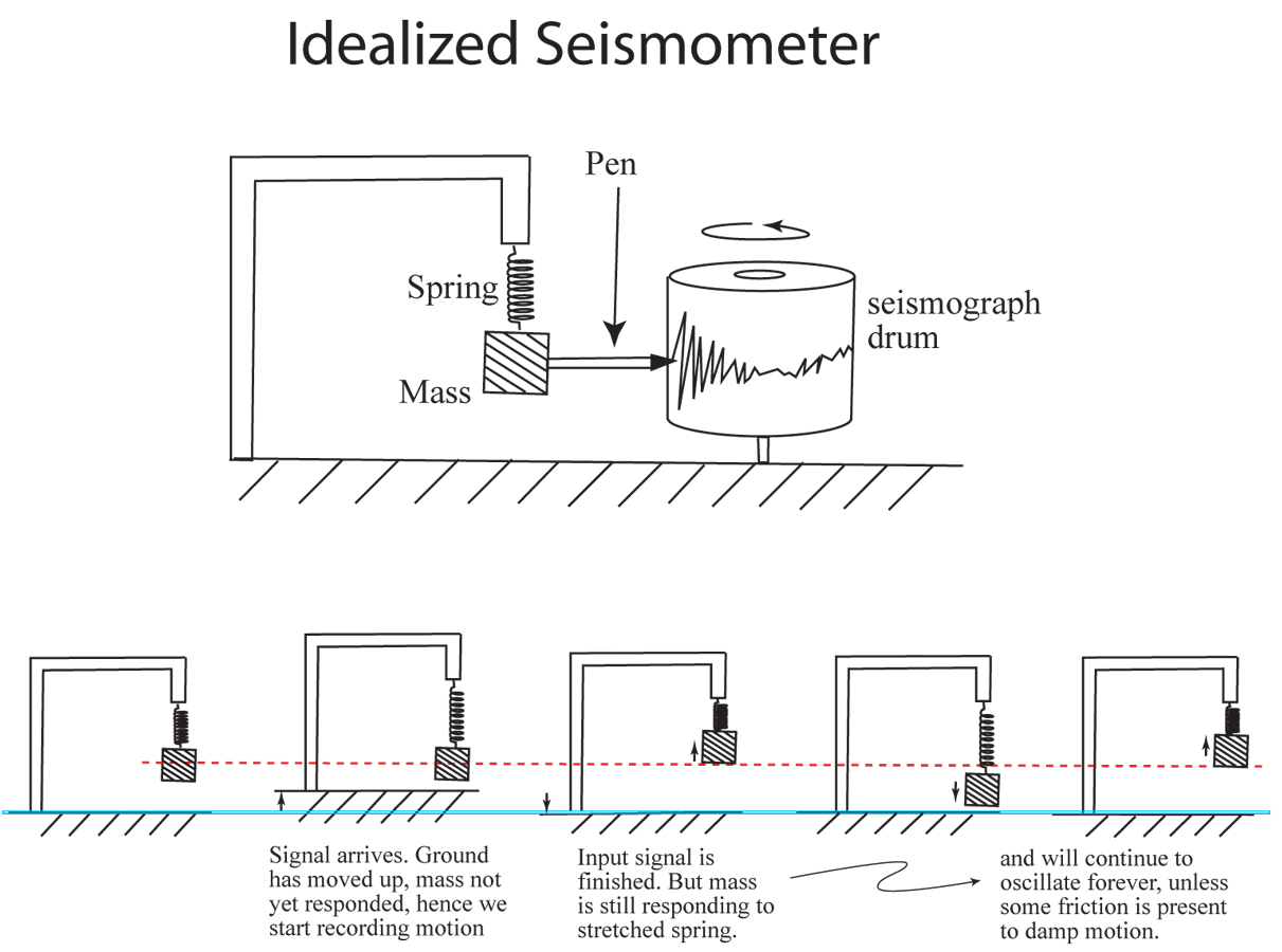
Here I try to illustrate how a seismic recorder, a seismometer, records ground motion. For a nice discussion of seismometers, see:
SEISMOMETER |
|
Introduction to seismology images (return to image directory page)
|
||||
 |
 |
 |
 |
 |
| AI (183 Kb) JPG (129 Kb) | AI (172 Kb) JPG (157 Kb) | AI (213 Kb) JPG (177 Kb) | AI (164 Kb) JPG (97 Kb) | AI (132 Kb) JPG (105 Kb) |
|
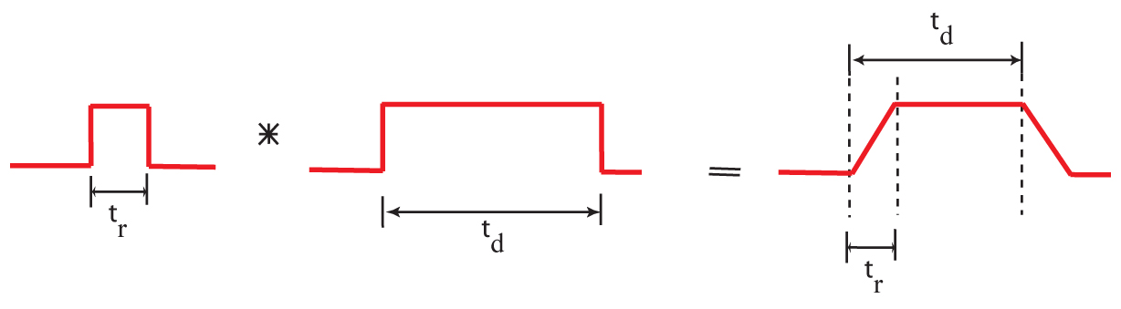
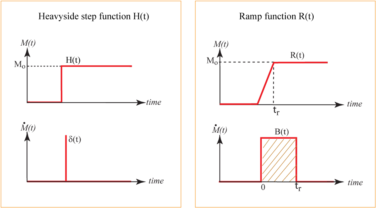
Seismic moment and moment rate functions are shown for the Heavyside and Ramp functions. See also:
SEISMIC MOMENT |
More on seismic moment.
|
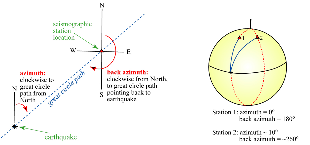
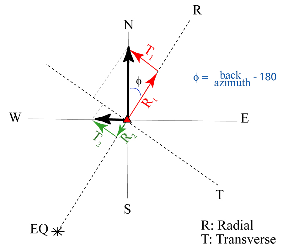
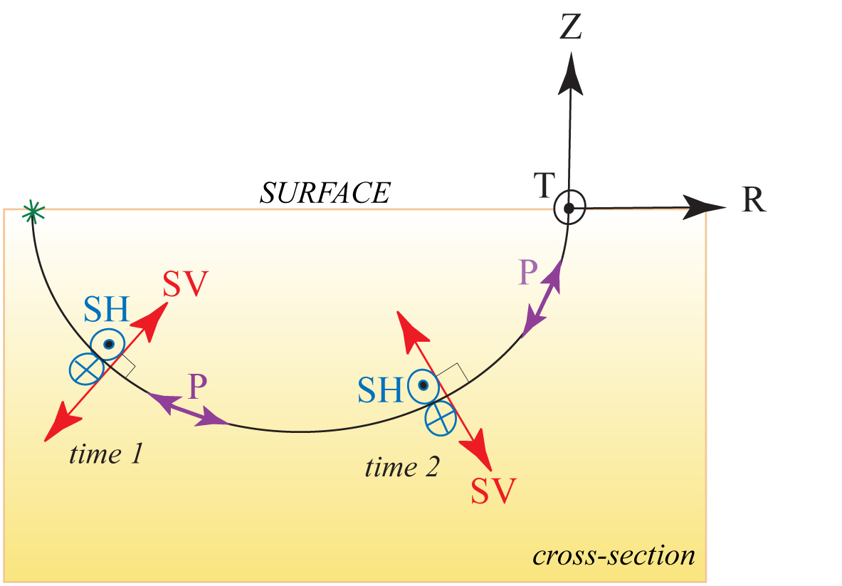
Here we define some orientation terms regarding seismic ray path from the earthquake to the seismometer.
|
Zooming into the location of the seismometer, we see the projection of the North-South and East-West components of motion onto the great-circle plane (for the radial, or R component) and perpendicular to it, the tangential, or T, component.
|
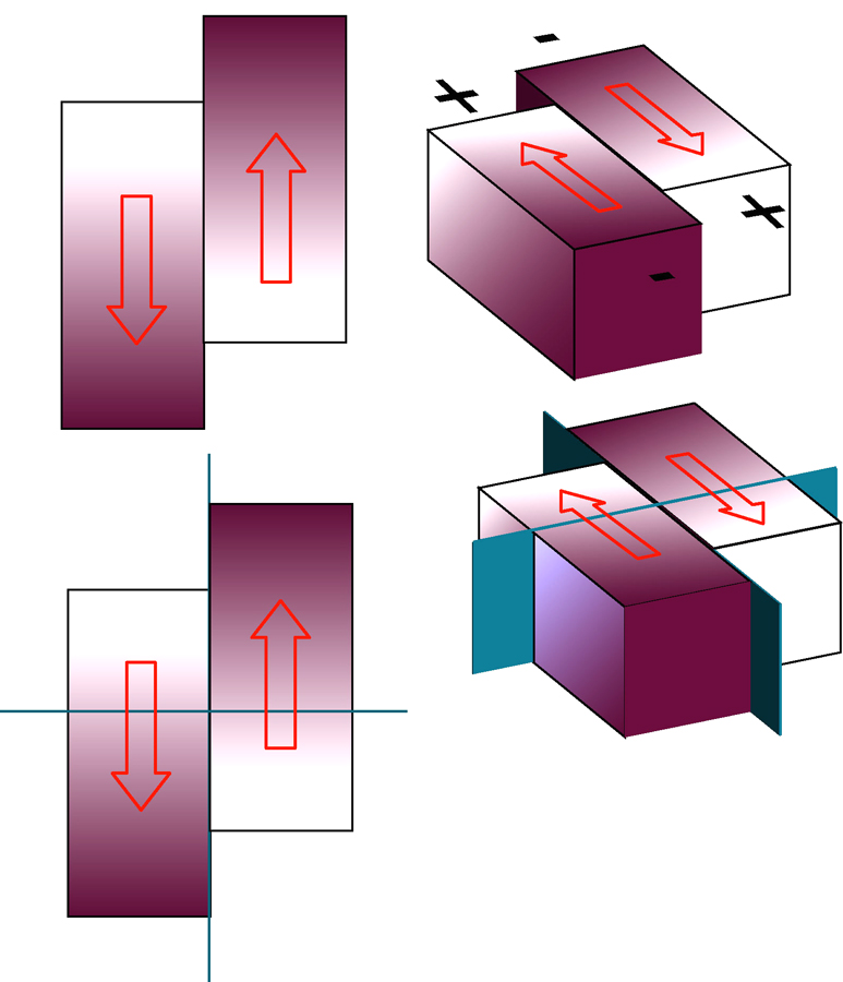
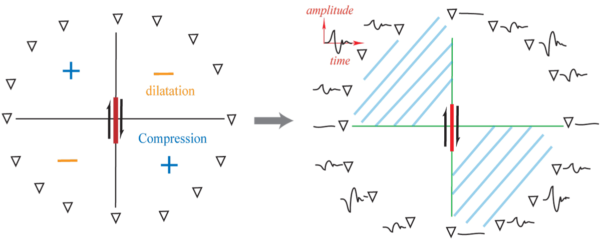
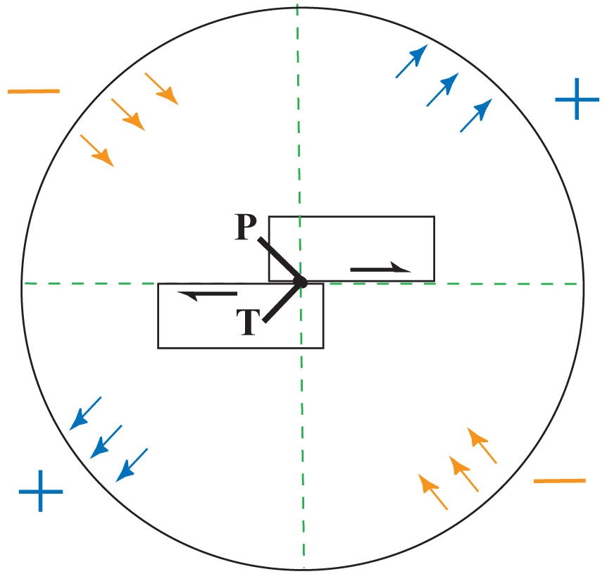
Slip on some fault blocks gives compressiive (blue) and tension (orange) motions in the far-field. Right at the source (in vicinity of slip), Tension (T) and compression (P) are experienced.
|
|
Introduction to seismology images (return to image directory page)
|
||||
 |
 |
 |
 |
 |
| AI (177 Kb) JPG (175 Kb) | AI (187 Kb) JPG (180 Kb) | AI (145 Kb) JPG (119 Kb) | AI (179 Kb) JPG (169 Kb) | AI (176 Kb) JPG (104 Kb) |
|
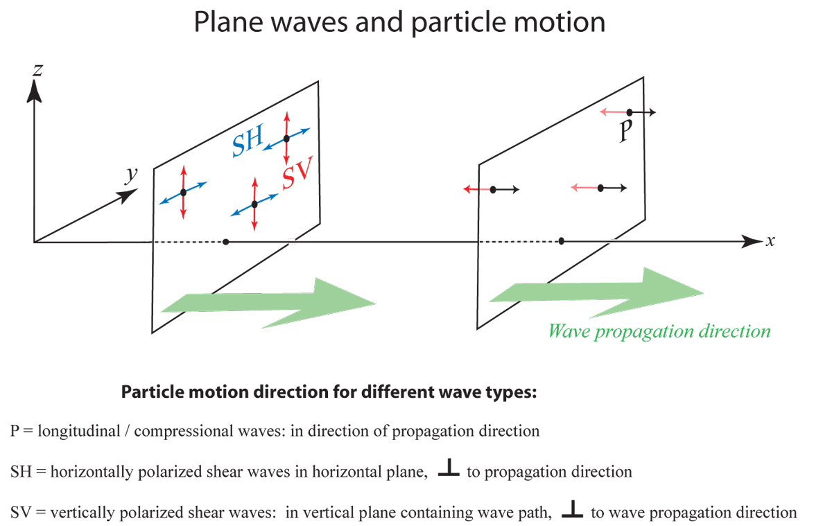
P-wave velocity (Vp) is always greater than S-wave velocity (Vs), hence P-waves arrive first. S-waves are further decomposed into SH and SV motions, which this figure defines.
|
This diagram pretty much shows the same thing as the last one, that is, the particle motion of some point as a P or SH or SV wave passed through that point.
|
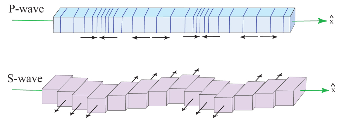
This is my version of the kind of image you find in a geology 101 textbook. The P-wave and S-wave (SH, actually) vibrate rock in specific directions depending on the wave propagation direction.
|
The main reason for separately studying SV and SH waves, is that if the medium is anisotropic, that is, seismic properties depend on propagation direction, then SH and SV will travel at different speeds.
|
I always loved the famous image used in Officer's geophysics book. I redrew some parts of it in this and the next image.
|
|
Introduction to seismology images (return to image directory page)
|
||||
 |
 |
 |
 |
 |
| AI (187 Kb) JPG (90 Kb) | AI (186 Kb) JPG (195 Kb) | AI (159 Kb) JPG (69 Kb) | AI (182 Kb) JPG (214 Kb) | AI (181 Kb) JPG (181 Kb) |
|
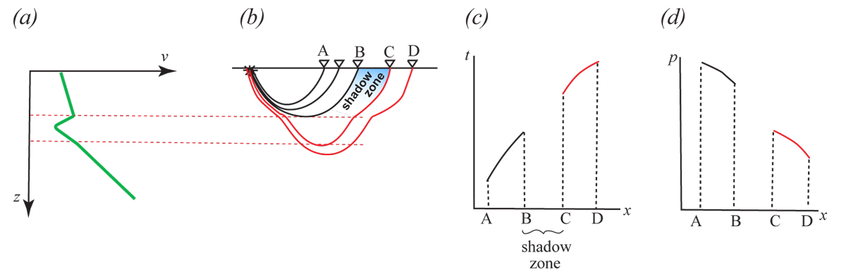
A low velocity zone results in a shadow zone (a region where no energy is transmitted to).
|
More of the same, but showing a few options all on the same figure.
|
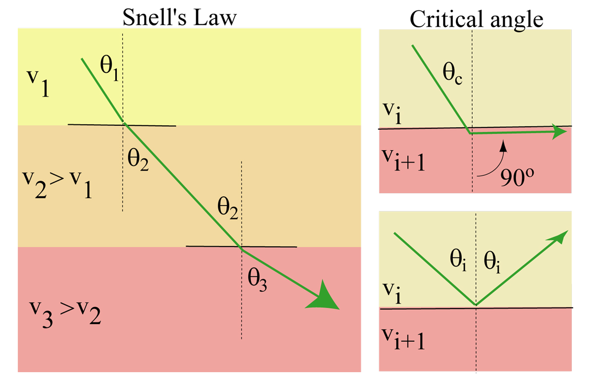
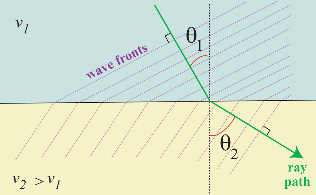
This is the simplest of my Snell's Law images. Snell's Law refers to how the seismic ray path (i.e., the normal to the wavefront) bends as you cross from one medium to another, according to the angle of approach and a ratio of the velocities.
|
Here we've just added the plane wavefronts. See also:
SNELL'S LAW REFRACTION |
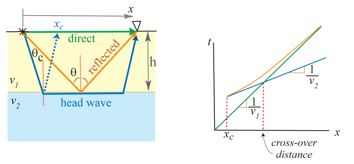
There is an angle, the critical angle, that defines the steepest incident angle that allows for transmission into the lower medium. It makes a wave called a head wave that travels along the interface
|
|
Introduction to seismology images (return to image directory page)
|
||||
 |
 |
 |
 |
 |
| AI (183 Kb) JPG (152 Kb) | AI (265 Kb) JPG (314 Kb) | AI (211 Kb) JPG (227 Kb) | AI (189 Kb) JPG (111 Kb) | AI (170 Kb) JPG (147 Kb) |
|
Simply another image emphasizing Snell's law and refraction of a wave through a layered medium, in Cartesian coordinates. Here's an animation of it: GIF (40 Kb)
|
Okay, this is overkill. Whatever. Maybe someone will find it useful...
|
This is a LOT like the image in the row above, except the wave is traveling downwards.
|
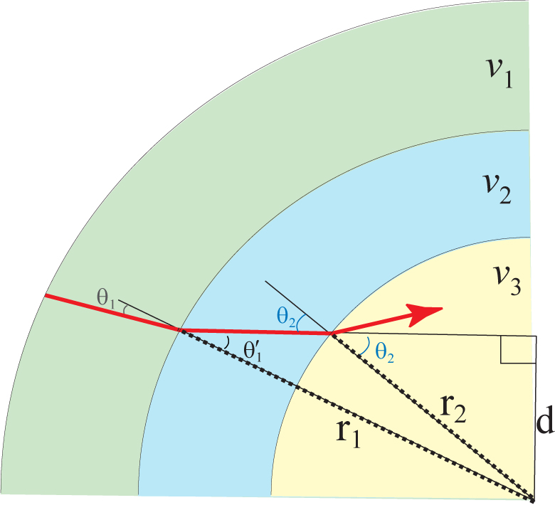
Snell's law is used in Spherical Coordinates also.
|
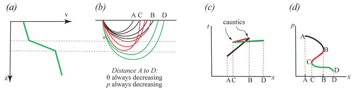
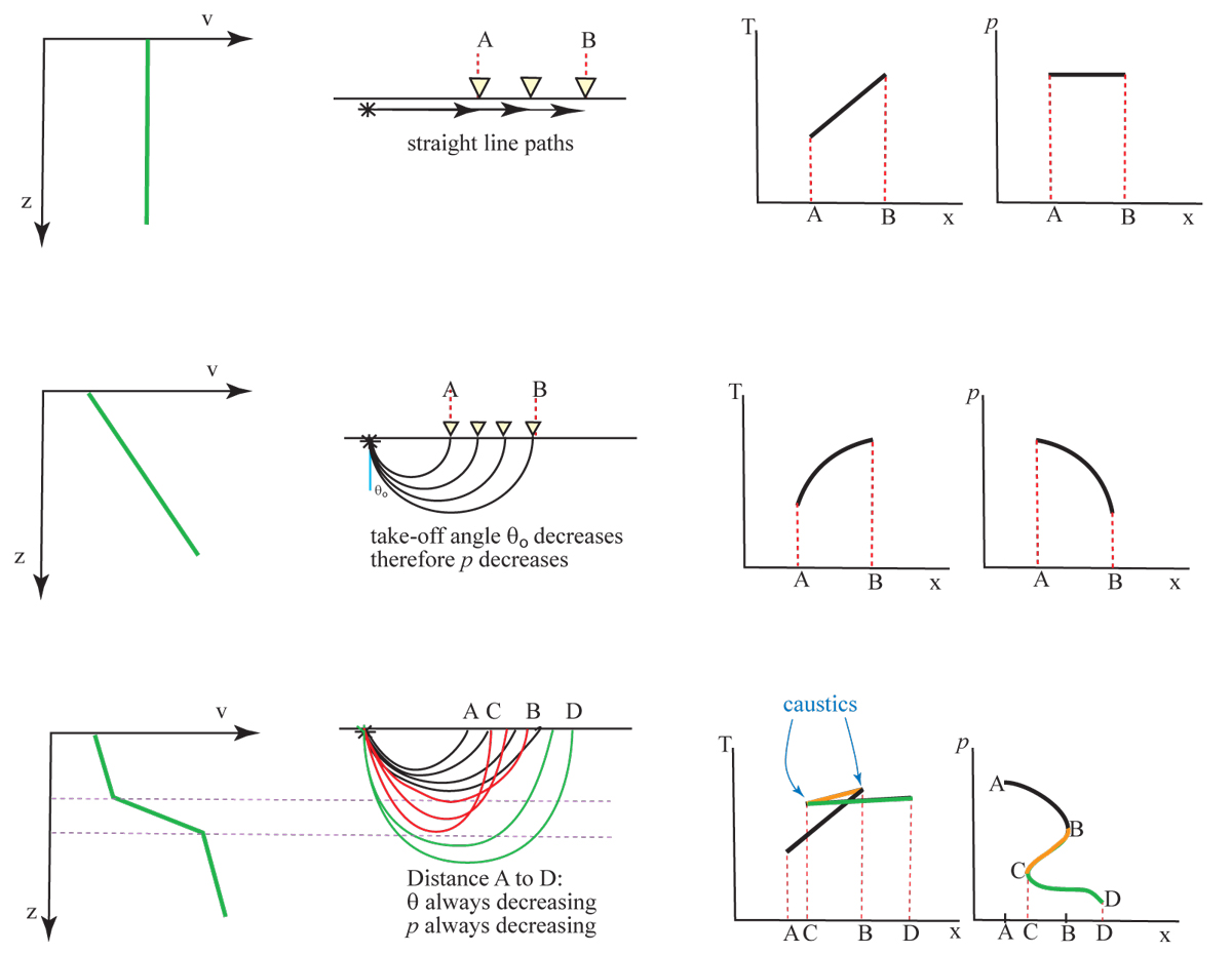
A layer on top of a higher velocity material results in 3 possible wave types, shown on the left, and in travel time we have 3 corresponding lines (or "branches") that together are called a triplication.
|
|
Introduction to seismology images (return to image directory page)
|
||||
 |
 |
 |
 |
 |
| AI (179 Kb) JPG (162 Kb) | AI (157 Kb) JPG (159 Kb) | AI (225 Kb) JPG (232 Kb) | AI (204 Kb) JPG (90 Kb) | AI (163 Kb) JPG (77 Kb) |
|
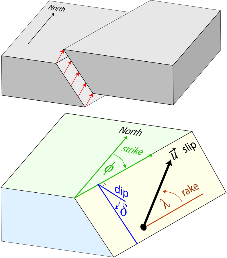
Here we define strike. dip, rake, and slip, in the so-called Aki & Richards convention. These terms fully define slip on a fault plane of some geometry.
|
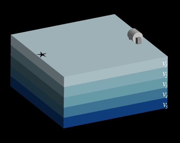
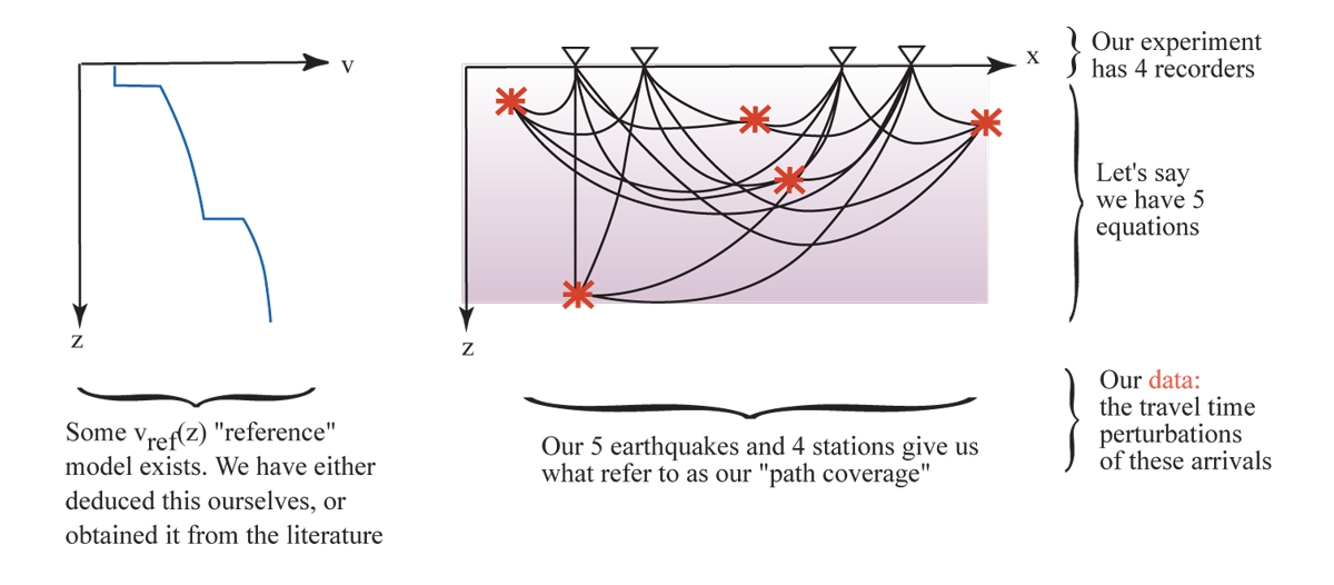
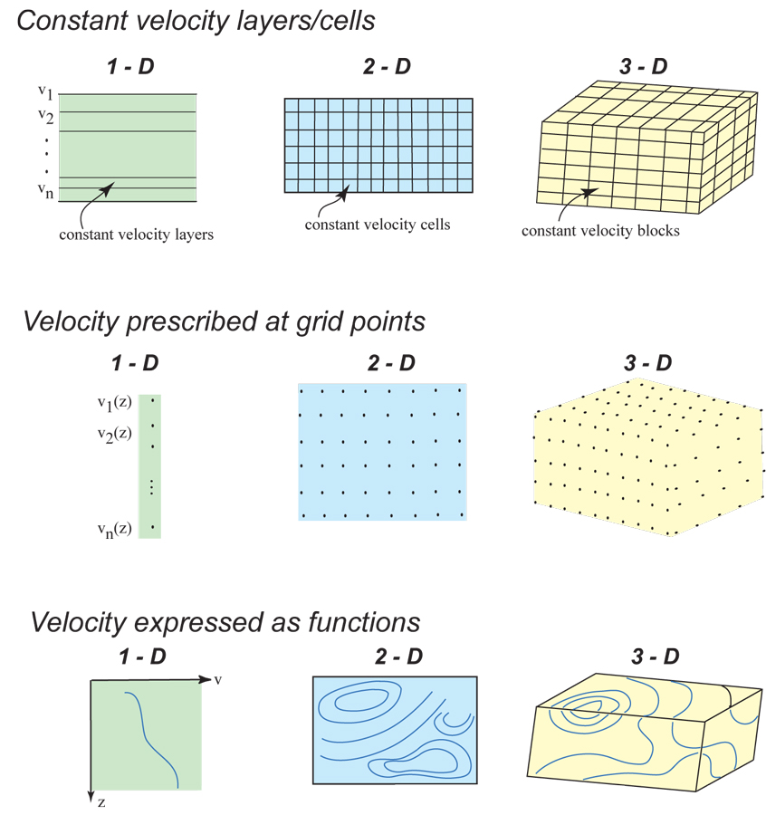
Seismic Tomography is the field that concerns itself with inverting lots and lots of seismic data to yield an image of the interior. To do this propertly, we need lots of earthquakes and lots of recorders.
|
The seismic tomography has to decide ahead of time how to set up the problem. This image shows several possibilities. Here's a PowerPoint file that illustrates the tomographic method using ultrasound PPT (575 Kb)
|
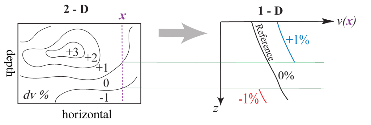
Here we look at a 2D cross-section with some velocity model (imagined to be from tomography), and how we interpret a 1D velocity-depth slice.
|
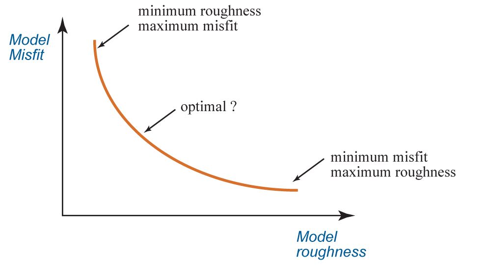
As with any inversion problem in mathematics, there are strong trade-offs. This image is meant to illustrate the classic trade-off between model roughness and misfit.
|
|
Introduction to seismology images (return to image directory page)
|
||||
 |
 |
 |
 |
 |
| AI (181 Kb) JPG (89 Kb) | AI (211 Kb) JPG (230 Kb) | AI (155 Kb) JPG (251 Kb) | AI (194 Kb) JPG (294 Kb) | AI (161 Kb) JPG (251 Kb) |
|
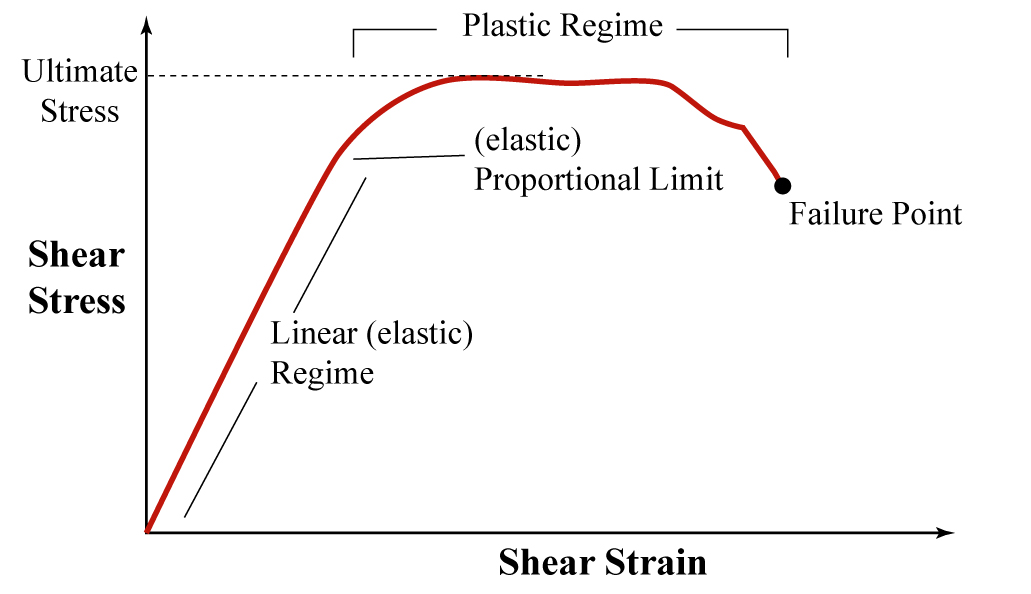
Stress and resulting strain is depicted for some medium. Most of seismology concerns itself in the linear part of the curve.
|
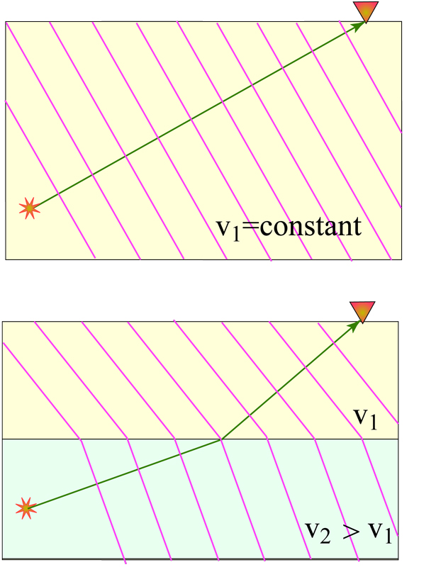
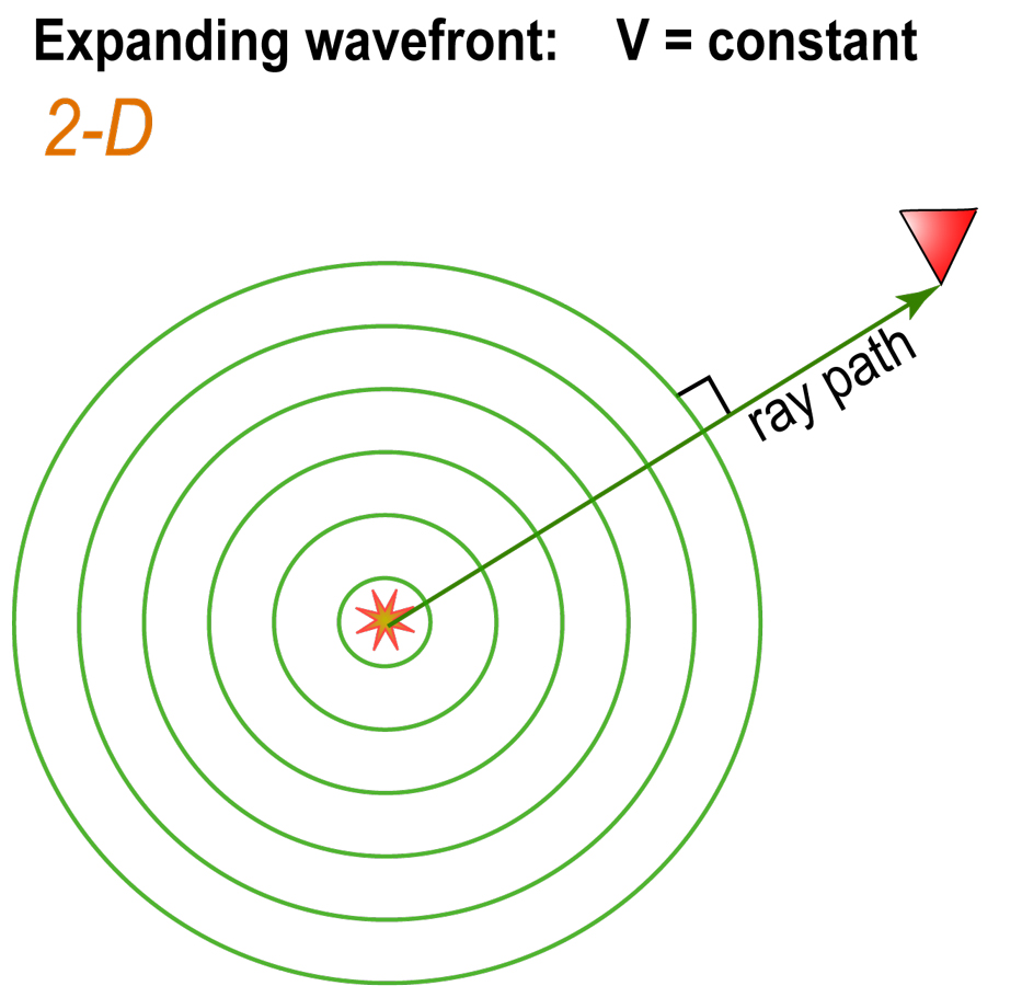
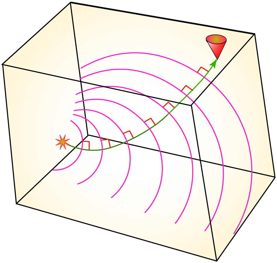
Yes, this is a "starting at square 1" image, to define the ray path as a normal to the wave front (circular in this case).
|
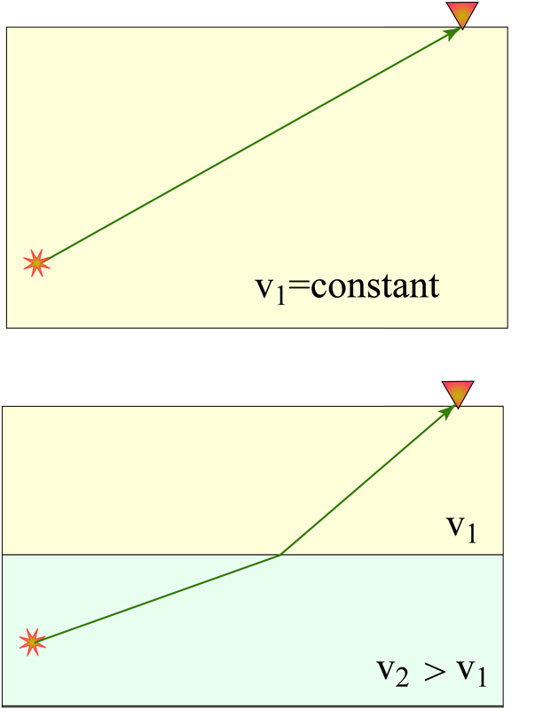
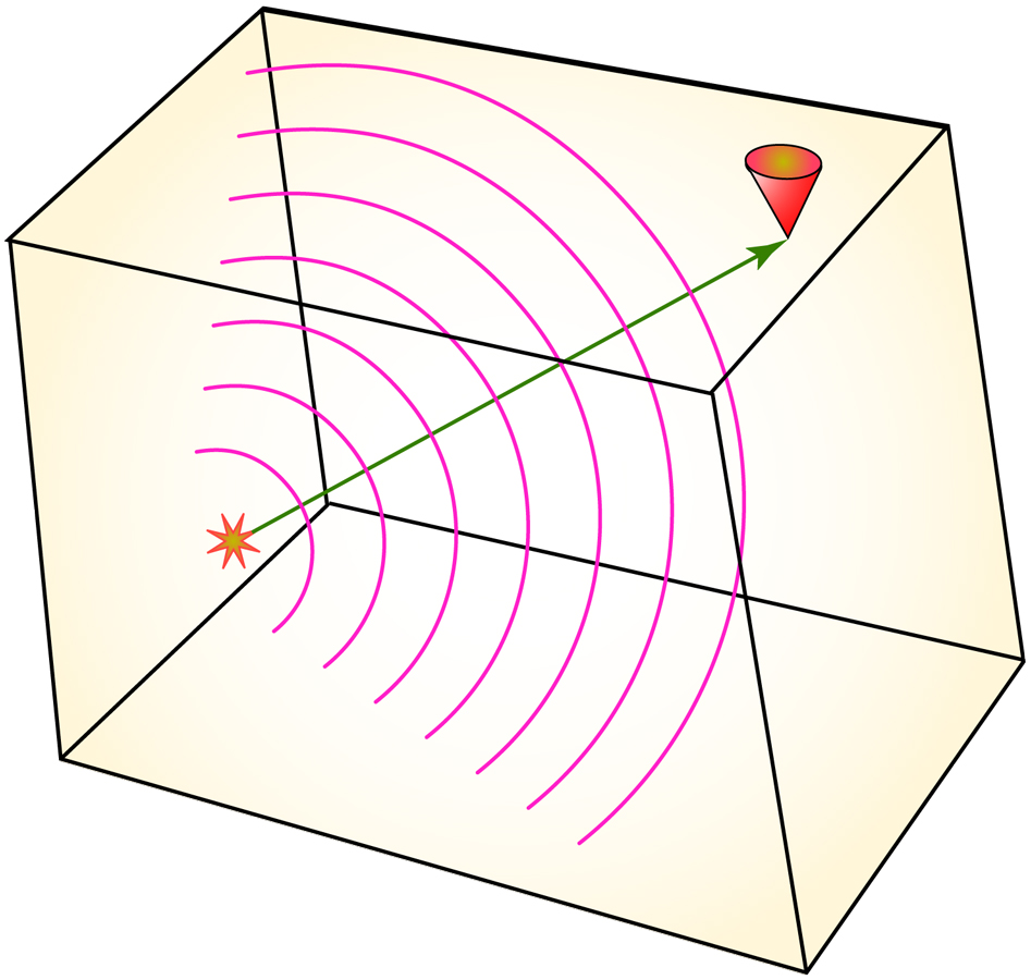
Same thing as the last figure, but in a constant velocity box.
|
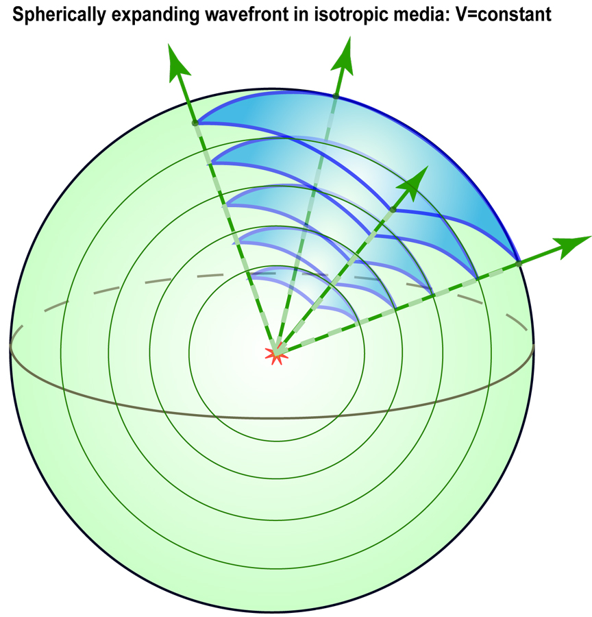
I'm scratching my head wondering why I made this figure. I think it was to illustrate geometric spreading (since the same cone of energy fills an increasing area, you get diminishing amplitudes).
|
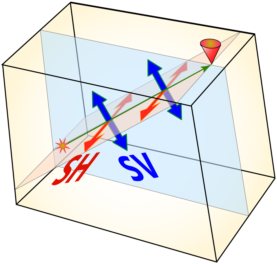
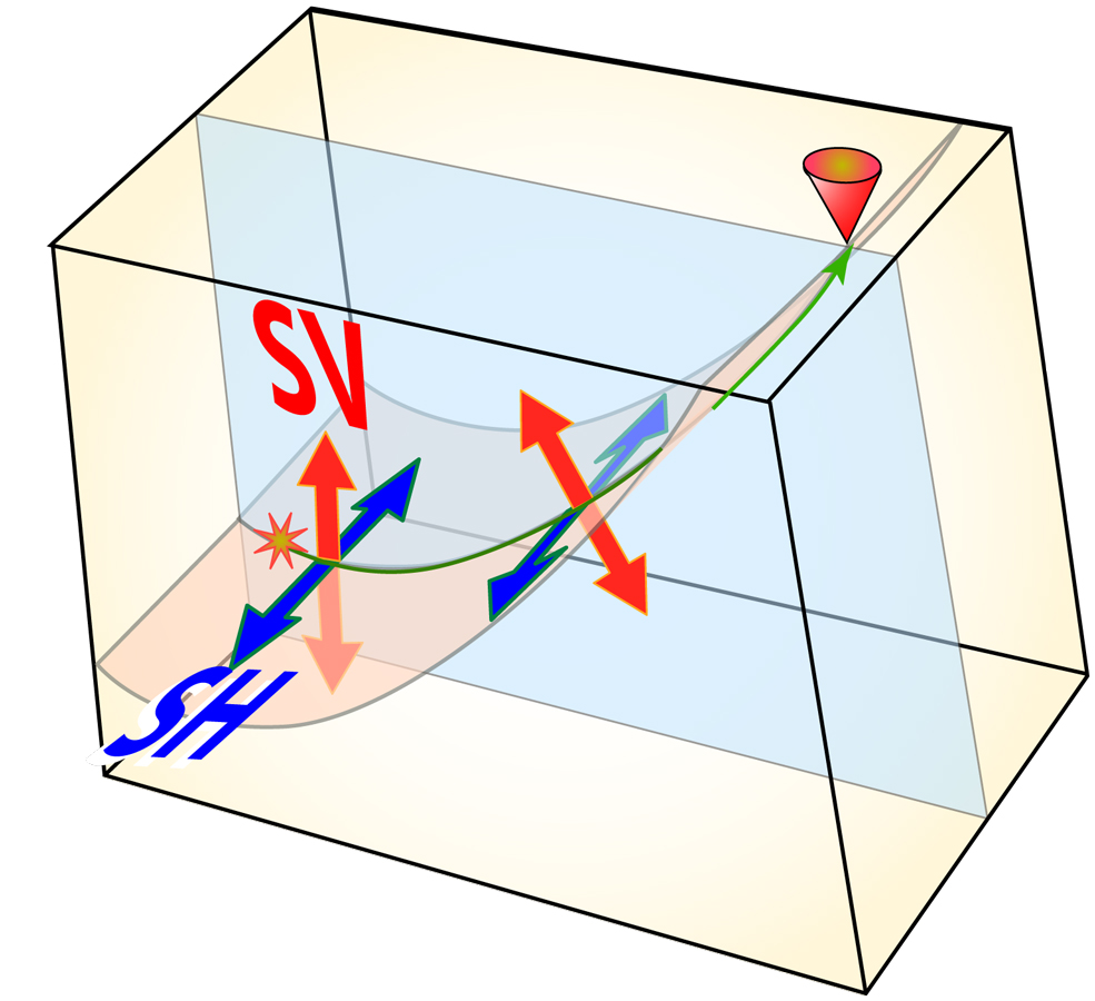
This should be about 4 rows up... Anyway, we see the SH and SV particle motion directions for a constant velocity medium.
|
|
Introduction to seismology images (return to image directory page)
|
||||
 |
 |
 |
 |
 |
| AI (143 Kb) JPG (251 Kb) | AI (150 Kb) JPG (246 Kb) | AI (200 Kb) JPG (144 Kb) | AI (643 Kb) JPG (262 Kb) | JPG (210 Kb) |
|
In this box, the velocity increases with depth. This results in a distortion of the expanding spherical wavefronts, and hence the "ray path", i.e., the normal to the wavefronts, is bent.
|
Much like the last image in the row above, except the velocity is increasing with depth.
|
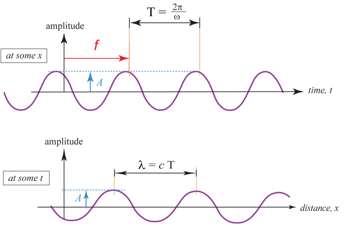
Here is my "wave basics" image. It is essentially a redrawing from an image in Bruce Bolt's intro book "Inside the Earth". My very 1st geophysics class was from Bolt, and about a week into it, I changed my major from geology to geophysics!
|
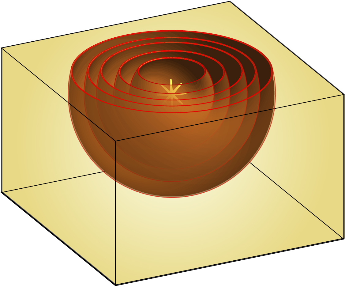
Just in case someone has trouble visualizing a wave front as expanding spheres, I made this image. Though I can't imagine there being such a person. Or maybe this was during my phase of making drink cups from old coconut shells for Helmberger's group meetings.
|
Mantle, outer core, inner core? Other than the inner core being too big, it's not too bad, eh?
|