
Images relating to seismic anisotropy in Earth's mantle
|
Some images relating to seismic anisotropy in Earth's interior (return to image directory page)
|
||||
 |
 |
 |
 |
 |
| AI (177 Kb) JPG (254 Kb) | AI (262 Kb) JPG (251 Kb) | AI (173 Kb) JPG (307 Kb) | AI (220 Kb) JPG (298 Kb) | AI (527 Kb) JPG (322 Kb) |
|
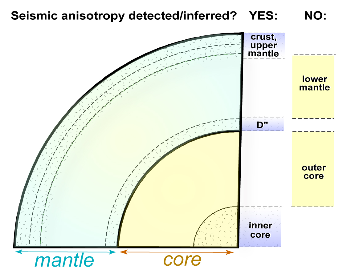
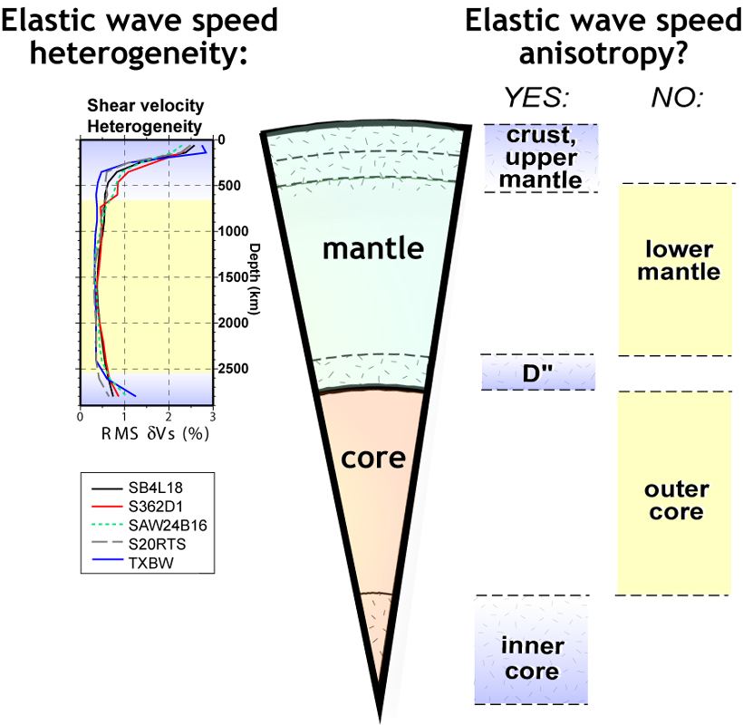
This is a simple figure showing different depth shells within Earth for which seismic anisotropy has been reported.
|
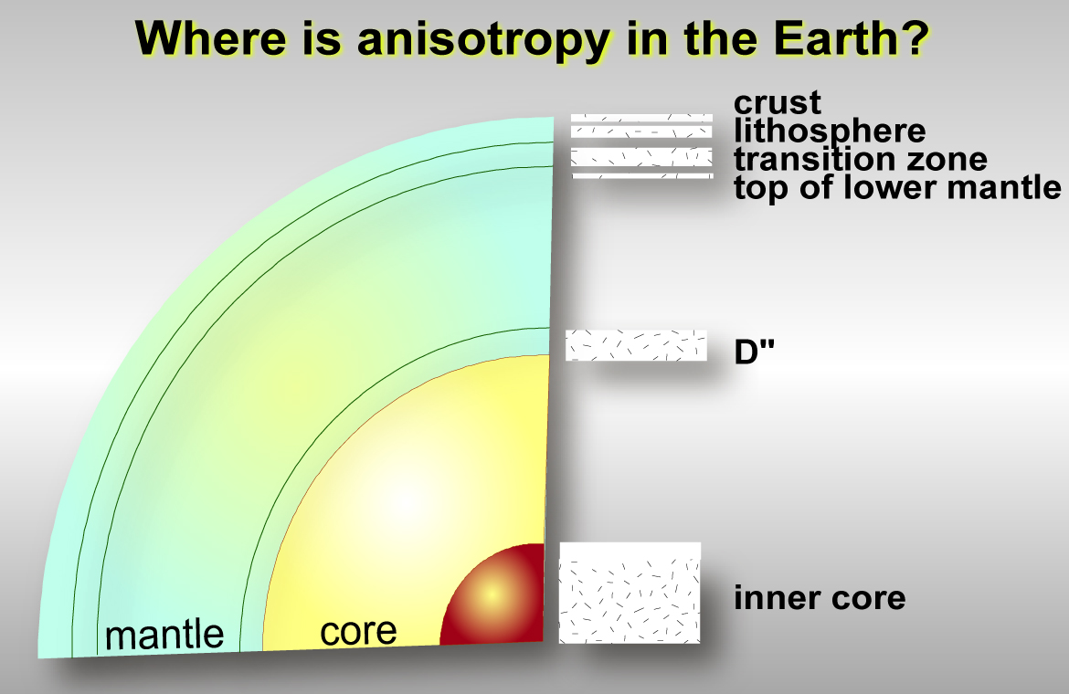
Here is another version of the figure to the left. This figure more specifically hints at the possibility that the outermost inner core might be isotropic, and the top of the lower mantle might be anisotropic.
|
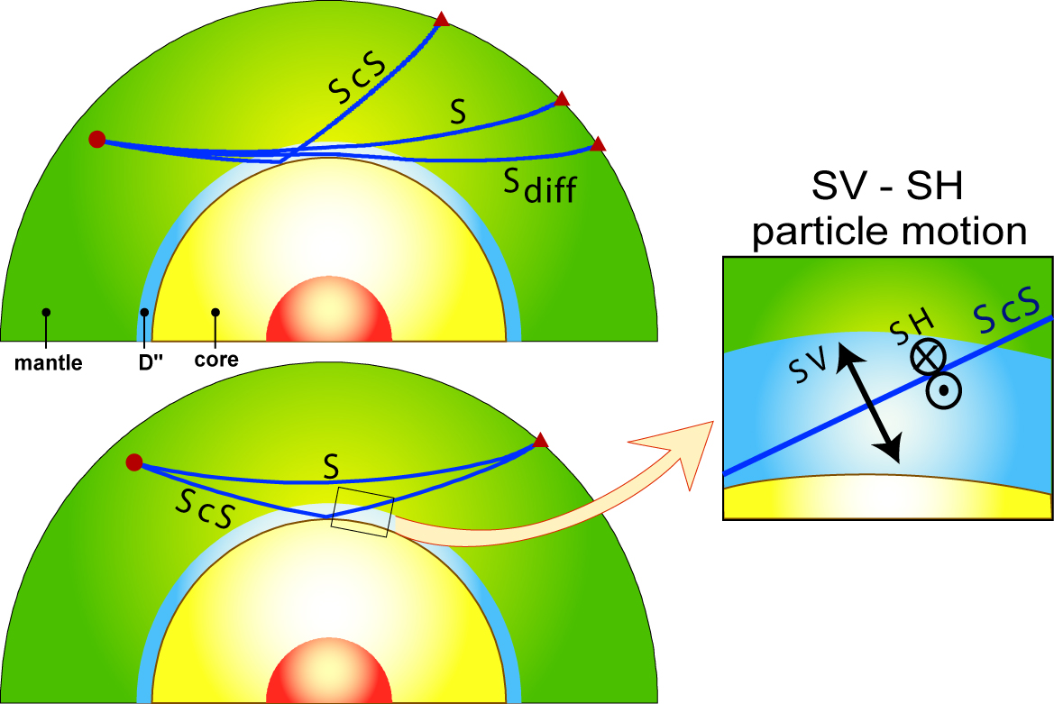
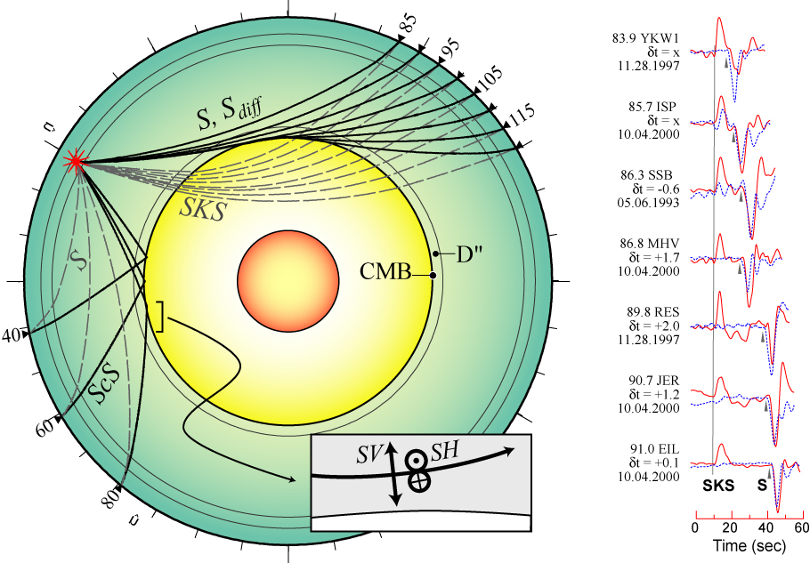
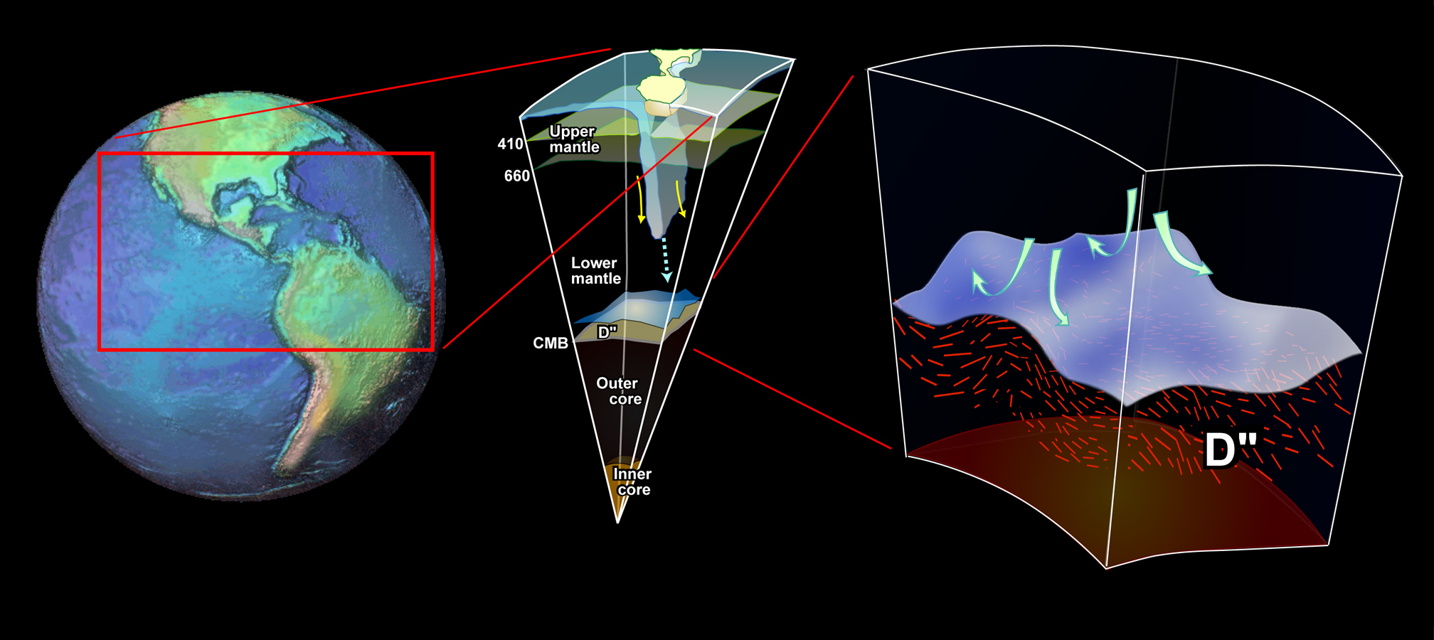
The most commonly used probes of deep mantle seismic anisotropy are displayed, with a zoom of the D" region showing the SV and SH particle motion.
|
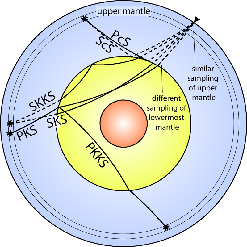
If the deepest mantle is anisotropic, then it may affect waves used to study upper mantle anisotropy (and visa versa). This figure was from a proposal aimed at studying both simultaneously (it didn't get funded... oh well).
|
Fairly similar to 2 panels to the left, this figure also shows some SKS and S wave data (SV traces are red, SH blue). Since SKS is close to S at the closer distances, it is hard to resolve the depth of the onset of D" anisotropy.
|
|
Some images relating to seismic anisotropy in Earth's interior (return to image directory page)
|
||||
 |
 |
 |
 |
 |
| AI (187 Kb) JPG (265 Kb) | AI (232 Kb) JPG (279 Kb) | AI (315 Kb) JPG (350 Kb) | AI (147 Kb) JPG (151 Kb) | AI (178 Kb) JPG (156 Kb) |
|
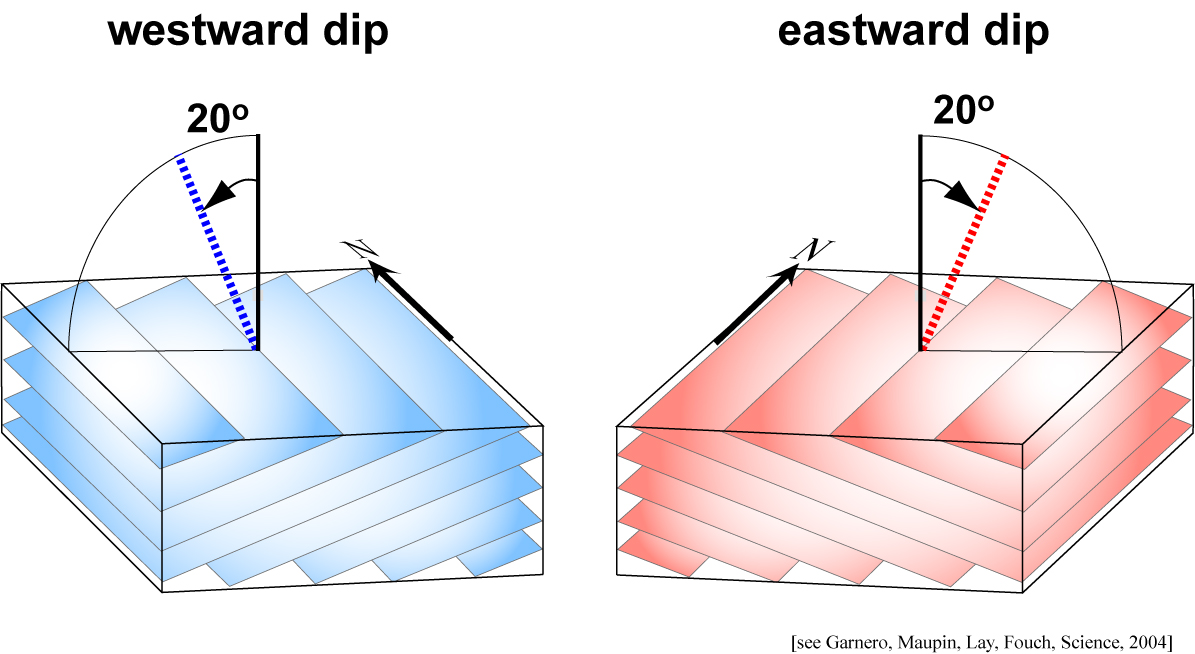
For our work under the Caribbean, stight tilts of the VTI symmetry axis either towards the east or west well-explained observed SV (or SVdiff) precursor behavior. [PDF]
|
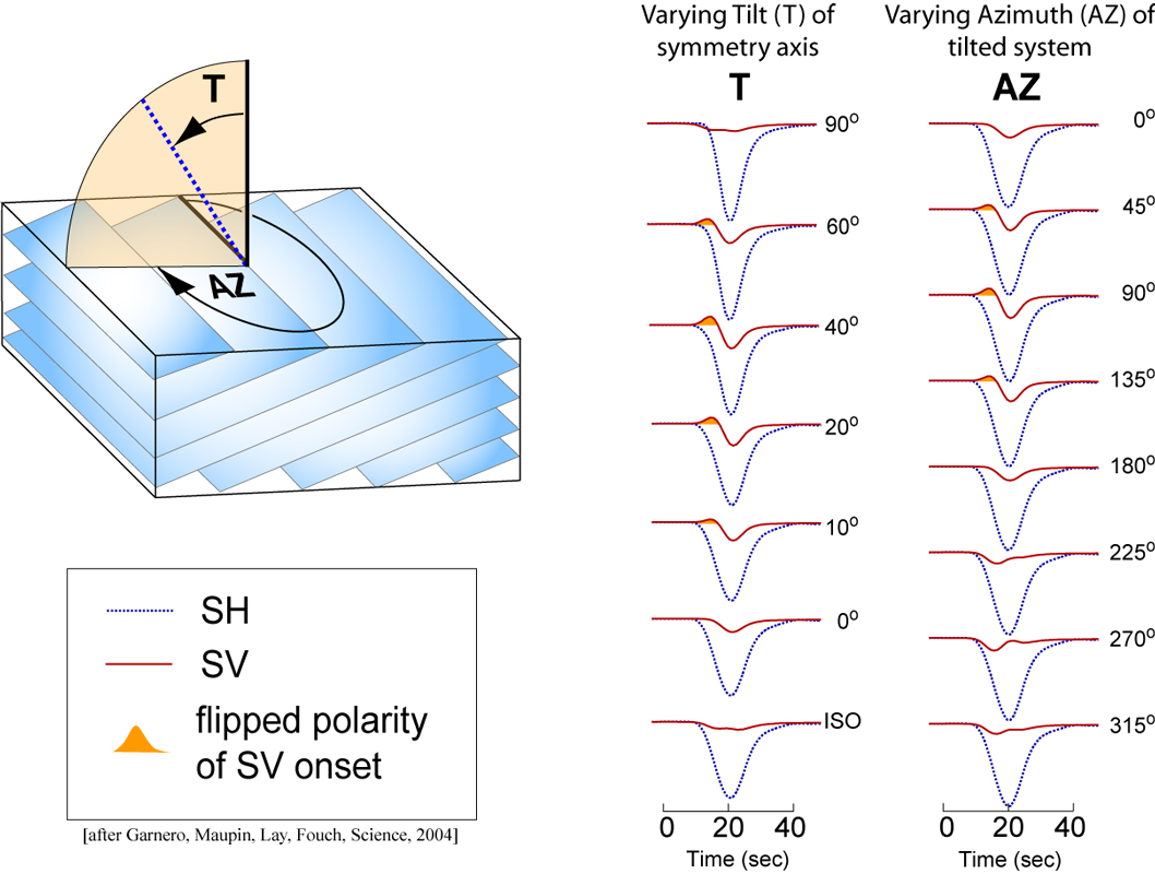
This figure shows how the SV component of S waves can cycle through different shapes depending on the tilt and azimuth of the transverse isotropy symmetry axis. [PDF]
|
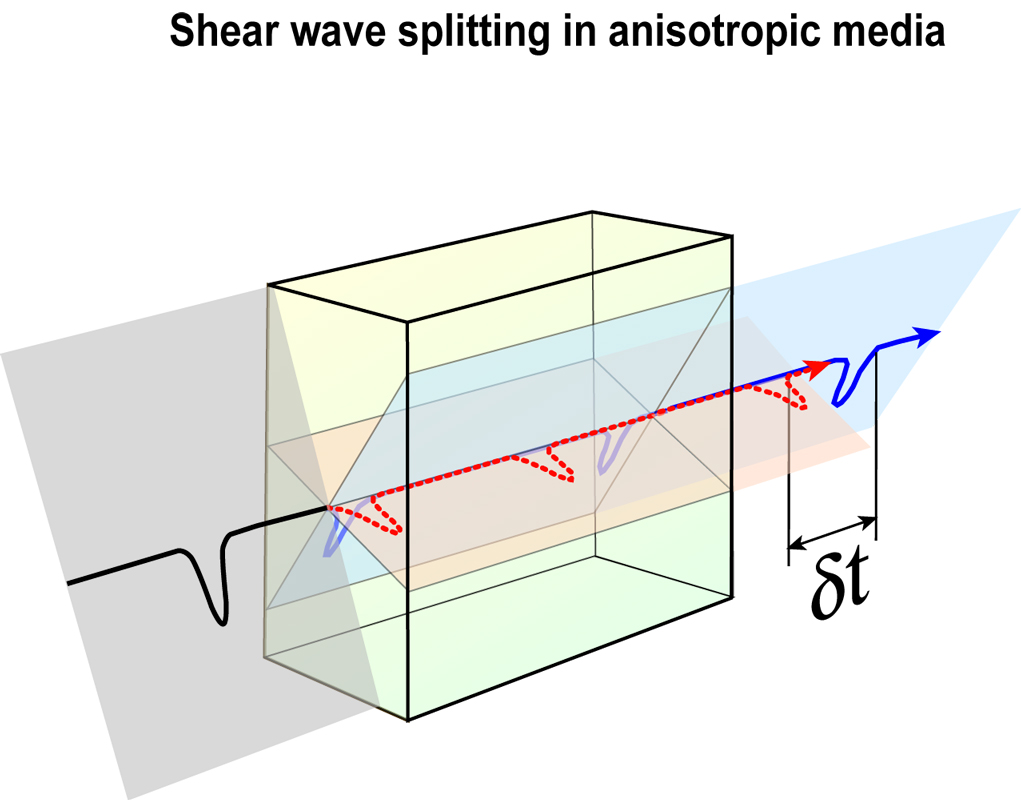
I basically redrew the famous Crampin (1981) figure, in color. The next two figures are simply differing presentations of the same. Here's a PowerPoint sequence of these images. Click HERE for an animation.
|
The blue pulses represent the faster wave, the red pulses the slower wave. They bifurcate upon encountering the anisotropic medium.
|
When the two pulses reach an observatory, seismologists measure the differential time and polarzation of the energy.
|
|
Some images relating to seismic anisotropy in Earth's interior (return to image directory page)
|
||||
 |
 |
 |
 |
 |
| AI (357 Kb) JPG (195 Kb) | AI (273 Kb) JPG (357 Kb) | AI (164 Kb) JPG (239 Kb) | AI (453 Kb) JPG (444 Kb) | AI (205 Kb) JPG (314 Kb) |
|
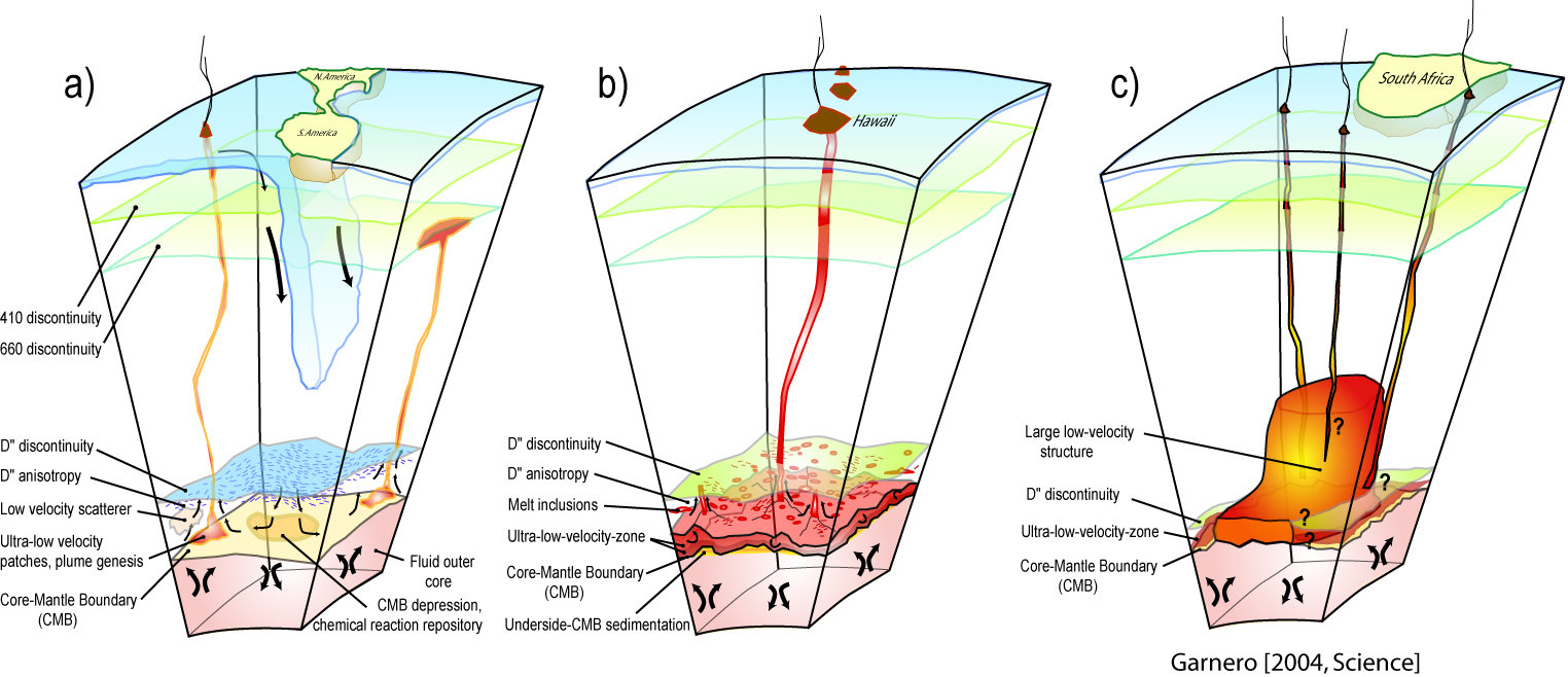
Here the connection is made between anisotropic and heterogeneous zones in the mantle: the "ends" of the mantle are the most heterogeneous, and possess the clearest evidence for anisotropy.
|
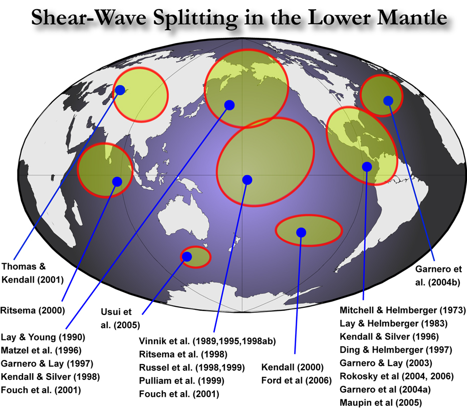
Regions where deep mantle anisotropy has been studied are shown. I apologize in advance if any work is missing from this figure (This figure needs updating!).
|
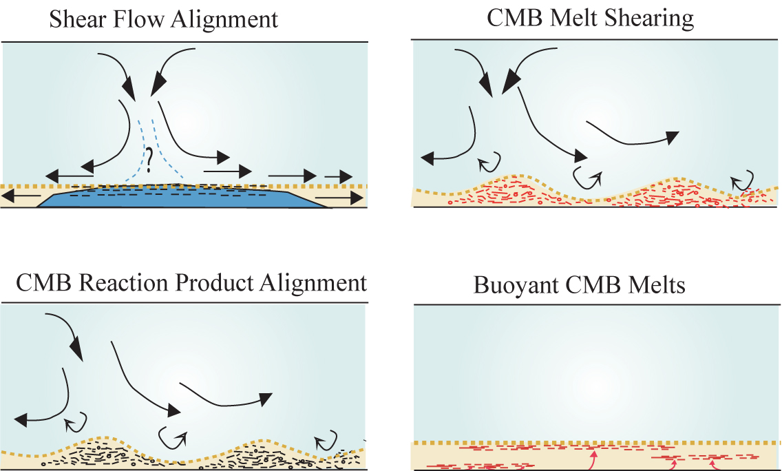
A variety of possibilities exist for the origin of seismic anisotropy (e.g., see reviews by Lay et al., 1998; and Kendall, 2000). Here, we speculate on some involving SPO (shape-preferred orientation) of materials. [PDF]
|
Both up- and down-welling regions show evidence for seismic anisotropy (middle and left panel, respectively). SPO and LPO (lattice-preferred orientation) have been discussed as causes to anisotropy in up and down-welling flow, respectively. [PDF]
|
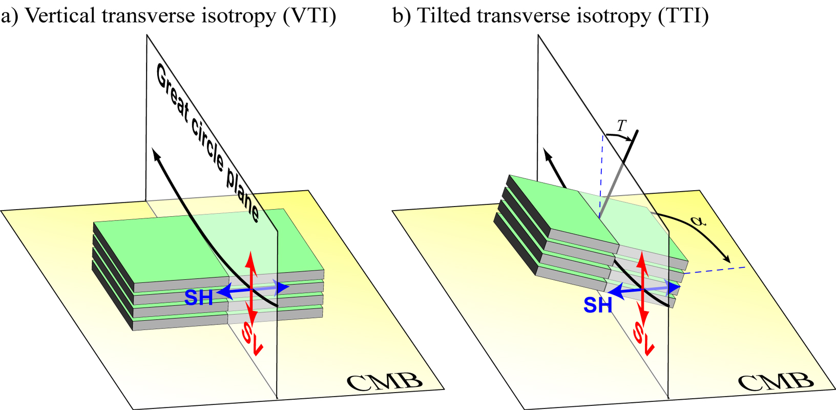
One form of azimuthal anisotropy is a tilt of the axis of symmetry of VTI (vertical transverse isotropy). This is a simple form of azimuthal anisotropy, as only two parameters are needed to describe the geometry (tilt and azimuth). [PDF]
|
|
Some images relating to seismic anisotropy in Earth's interior (return to image directory page)
|
||||
 |
 |
 |
 |
 |
| AI (778 Kb) JPG (265 Kb) | AI (128 Kb) JPG (232 Kb) | AI (5.0 Mb) JPG (421 Kb) | AI (774 Kb) JPG (163 Kb) | AI (214 Kb) JPG (238 Kb) |
|
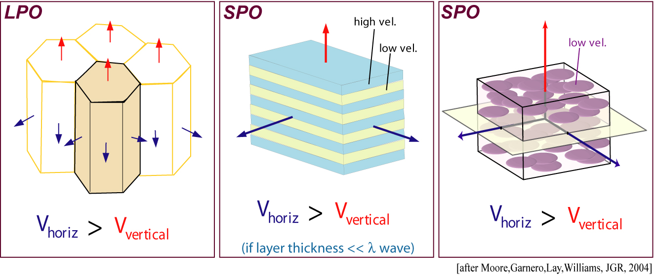
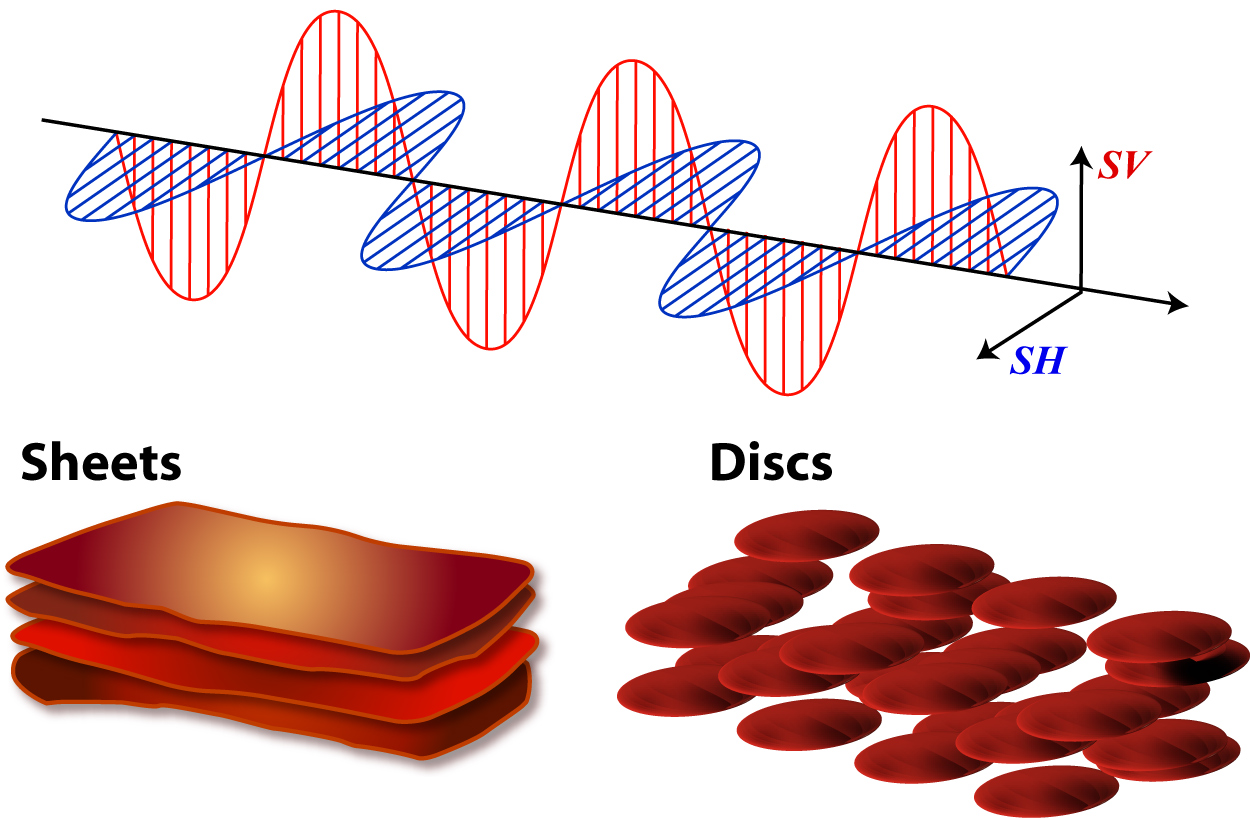
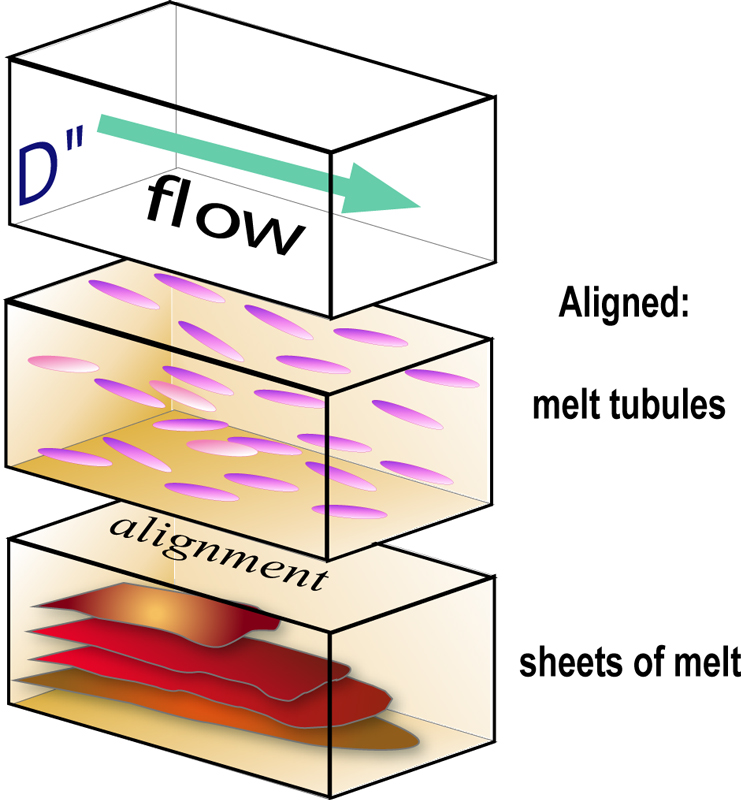
A variety of physical scenarios might give rise to either LPO or SPO. Here, we speculate on possibilities that result in waves with particle motion in the horizontal plane propogating faster than waves with vertical particle motion. [PDF]
|
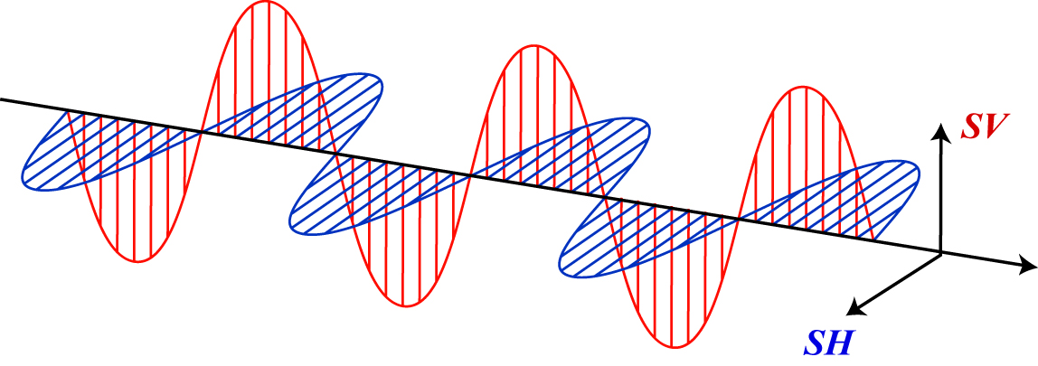
I've always liked the classic diagrams in physics books for electromagnetic waves, so I drew one for SV and SH particle motion.
|
So, why not throw in some fabric? Here we have sheets or flattened bubbles of melt.
|
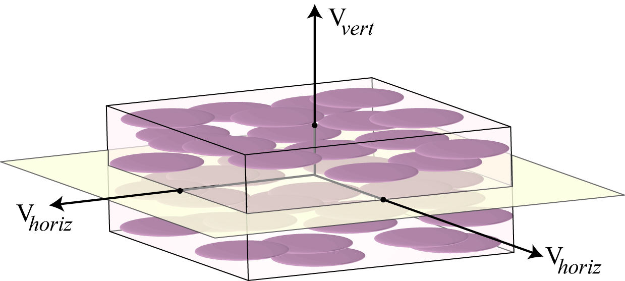
Just another depiction of flattened spherical inclusions.
|
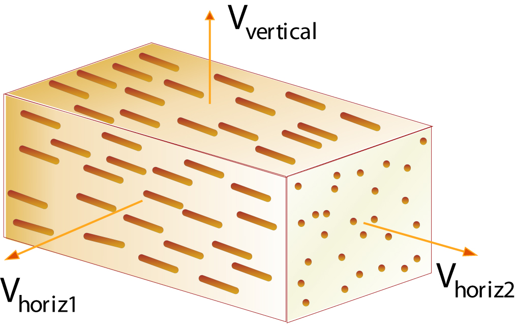
I probably shouldn't admit that I got the idea for this figure from a bar of soap with aligned lavendar pieces.
|
|
Some images relating to seismic anisotropy in Earth's interior (return to image directory page)
|
||||
 |
 |
 |
 |
 |
| AI (231 Kb) JPG (220 Kb) | AI (180 Kb) JPG (201 Kb) | AI (389 Kb) JPG (154 Kb) | PSD (16Mb) JPG (203 Kb) | JPG (486 Kb) |
|
Characterizing anisotropy is important, as it might one day permit us to map out dynamical flow in the lower mantle.
|
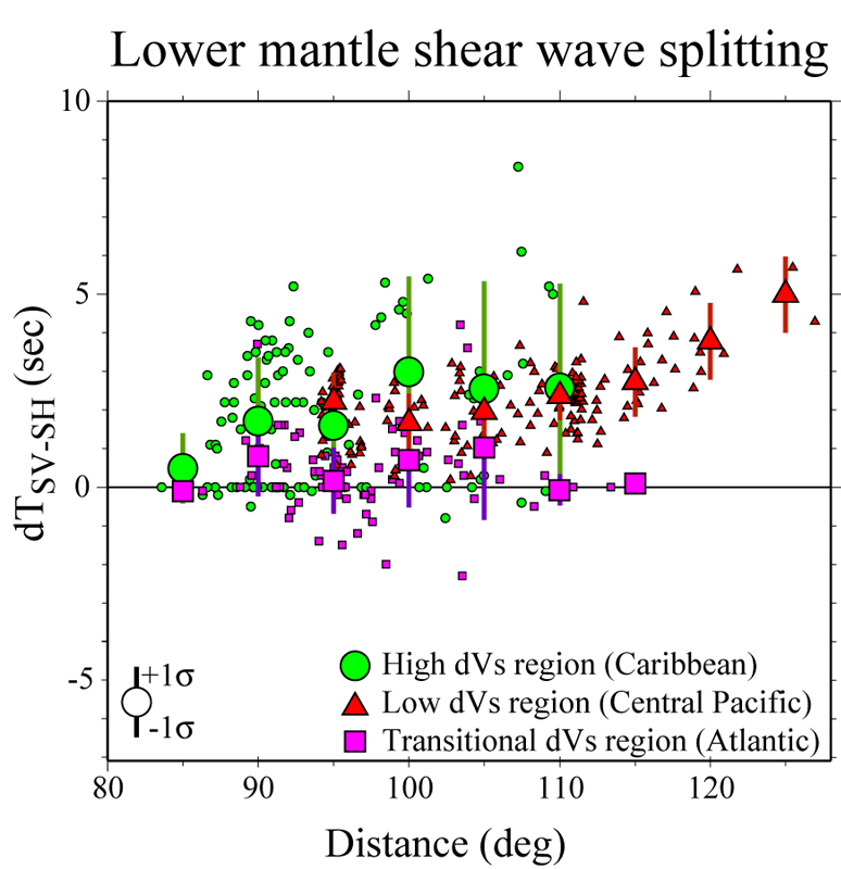
Travel times between the SV and SH components of motion of S and Sdiff waves are plotted versus epicentral distance. Larger symbols are distance bin averages. The down and upwelling regions show strong splitting, but a region presumably between up and down motions lacks strong splitting. [PDF]
|
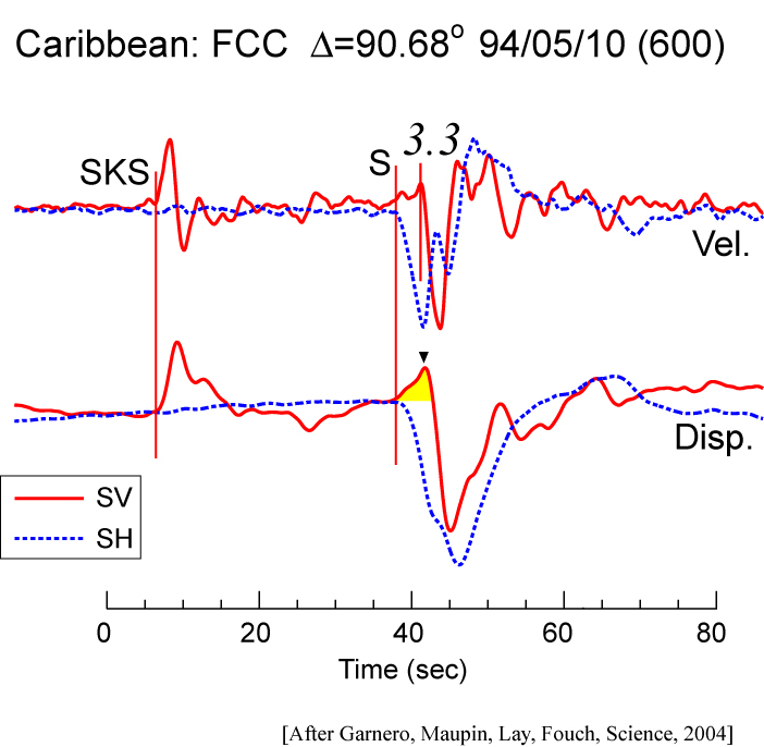
In measuring shear wave splitting, it is important to note that it may matter if you measure splits on the velocity (top) or displacement (bottom) traces -- here we show that velocity traces obscure the important SV waveform onset (yellow) used to map azimuthal anisotropy. [PDF]
|
I'm the first to admit this figure is a little overboard. Oh well, I was trying to get a certain journal to put it on their cover (unsuccesfully...). It shows a D" discontinuity (blue) underlain by a mid-D" layer (such as an exit from post-perovskite phase), and the CMB. Throw in some ULVZ melt for fun (red). [PDF]
|
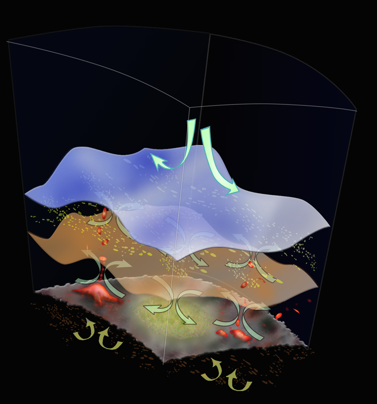
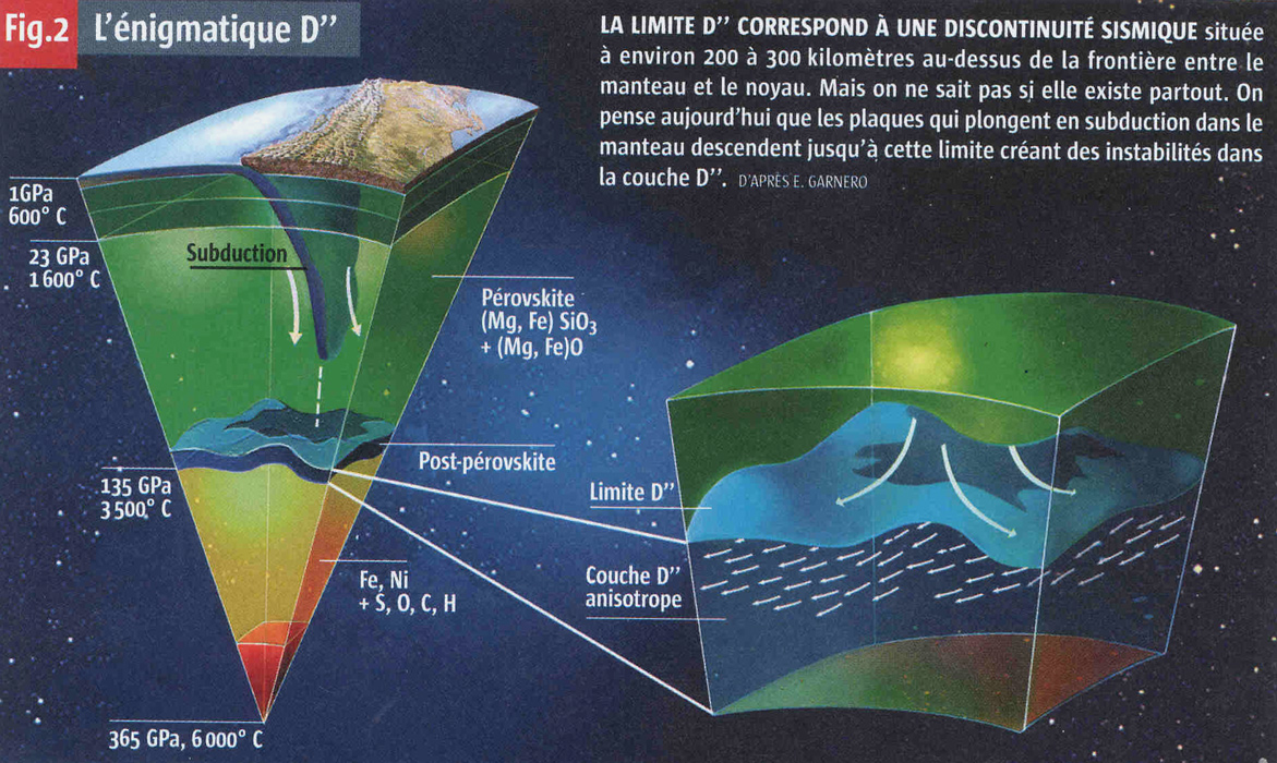
In this figure I was trying to emphasize that D" is subject to the whims of the overlying mantle: subduction currents can induce topography. Speak french? This is from La Recherche, (#382, Jan 2005) JPG (437 Kb). Obviously, real artists make much prettier pictures. [PDF]
|